27.13 Applications of RD Designs
Regression Discontinuity (RD) designs have widespread applications in empirical research across economics, political science, marketing, and public policy. These applications leverage threshold-based decision rules to identify causal effects in real-world settings where randomized experiments are infeasible.
Key applications include:
Marketing: Estimating the causal effects of promotions and advertising intensity.
Education: Evaluating the impact of financial aid or merit scholarships.
Healthcare: Assessing the effect of medical interventions assigned based on eligibility thresholds.
Labor Economics: Studying unemployment benefits and wage policies.
27.13.1 Applications in Marketing
RD has been widely applied in marketing research to estimate causal effects of pricing, advertising, and product positioning.
- Position Effects in Advertising
(Narayanan and Kalyanam 2015) uses an RD approach to estimate the causal impact of advertisement placement in search engines. Since ad placement follows an auction-based system, a discontinuity occurs where the top-ranked ad receives disproportionately more clicks than lower-ranked ads.
Key insights:
Higher-ranked ads generate more click-throughs, but this does not always translate into higher conversion rates.
The RD framework helps distinguish correlation from causation by leveraging the rank cutoff.
- Identifying Causal Marketing Mix Effects
(Hartmann, Nair, and Narayanan 2011) presents a nonparametric RD estimation approach to identify causal effects of marketing mix variables, such as:
Advertising budgets
Price changes
Promotional campaigns
By comparing firms just above and below an expenditure threshold, the RD framework isolates the true causal impact of marketing spending on consumer behavior.
27.13.2 R Packages for RD Estimation
Table 27.3 shows key RD Packages in R
| Feature | rdd | rdrobust | rddtools |
|---|---|---|---|
| Estimator | Local linear regression | Local polynomial regression | Local polynomial regression |
| Bandwidth Selection | (G. Imbens and Kalyanaraman 2012) | (Calonico, Cattaneo, and Titiunik 2014; G. Imbens and Kalyanaraman 2012 ; Calonico, Cattaneo, and Farrell 2020) | (G. Imbens and Kalyanaraman 2012) |
| Kernel Functions | Epanechnikov, Gaussian | Epanechnikov | Gaussian |
| Bias Correction | No | Yes | No |
| Covariate Inclusion | Yes | Yes | Yes |
| Assumption Testing | McCrary Sorting Test | No | McCrary Sorting, Covariate Distribution Tests |
For a detailed comparison, see Thoemmes, Liao, and Jin (2017) (Table 1, p. 347).
Specialized RD Packages
rddensity: Tests for discontinuities in the density of the running variable (useful for manipulation/bunching detection).rdlocrand: Implements randomization-based inference for RD.rdmulti: Extends RD to multiple cutoffs and multiple scores.rdpower: Conducts power calculations and sample selection for RD designs.
Why Use rdrobust?
- Implements local polynomial regression, providing bias correction and robust standard errors.
- Uses state-of-the-art bandwidth selection methods.
- Produces automatic RD plots for visualization.
27.13.3 Example of Regression Discontinuity in Education
We illustrate a Sharp RD using a simulated example of college GPA and future career success.
Setup:
Students qualify for a prestigious internship if their GPA ≥ 3.5.
The outcome variable is future career success (e.g., salary).
RD estimates the causal impact of the internship program on earnings.
\[ Y_i = \beta_0 + \beta_1 X_i + \beta_2 W_i + u_i \]
\[ X_i = \begin{cases} 1, W_i \ge c \\ 0, W_i < c \end{cases} \]
We simulate 100 observations, where GPA is the forcing variable and career success depends on GPA and the treatment effect.
# Set seed for reproducibility
set.seed(42)

n = 100

# Simulate GPA scores (0-4 scale)
GPA <- runif(n, 0, 4)

# Generate future success with treatment effect at GPA >= 3.5
future_success <- 10 + 2 * GPA + 10 * (GPA >= 3.5) + rnorm(n)

# Load RD package
library(rddtools)

# Format data for RD analysis
data <- rdd_data(future_success, GPA, cutpoint = 3.5)
Figure 27.4 shows the scatter plot of GPA and Future Success.
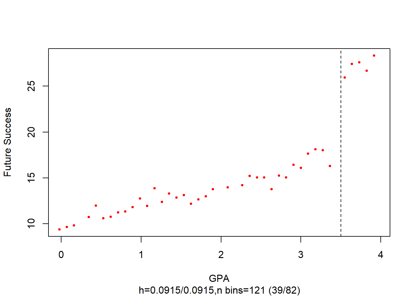
Figure 27.4: Binned Scatter Plot of GPA and Future Success with Threshold at 3.5
We estimate the Sharp RD treatment effect using local linear regression:
# Estimate the sharp RDD model
rdd_mod <- rdd_reg_lm(rdd_object = data, slope = "same")

# Display results
summary(rdd_mod)
#>
#> Call:
#> lm(formula = y ~ ., data = dat_step1, weights = weights)
#>
#> Residuals:
#>      Min       1Q   Median       3Q      Max
#> -3.08072 -0.54182  0.05352  0.54135  2.51267
#>
#> Coefficients:
#>             Estimate Std. Error t value Pr(>|t|)
#> (Intercept) 17.21703    0.20060   85.83   <2e-16 ***
#> D            9.79856    0.31716   30.89   <2e-16 ***
#> x            2.14839    0.09914   21.67   <2e-16 ***
#> ---
#> Signif. codes:  0 '***' 0.001 '**' 0.01 '*' 0.05 '.' 0.1 ' ' 1
#>
#> Residual standard error: 0.9284 on 97 degrees of freedom
#> Multiple R-squared:  0.9746, Adjusted R-squared:  0.9741
#> F-statistic:  1863 on 2 and 97 DF,  p-value: < 2.2e-16
Figure 27.5 plots the RD regression line with binned observations:
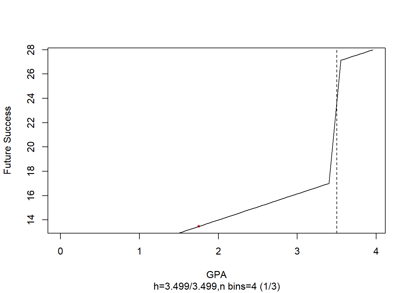
Figure 27.5: Coarse Binned Regression Discontinuity Plot of GPA and Future Success
We verify whether results hold under different bandwidths and functional forms:
- Varying the Bandwidth
# Using rdrobust for robust estimation
library(rdrobust)

# Estimate RD with optimal bandwidth
rd_out <- rdrobust(y = future_success, x = GPA, c = 3.5)
summary(rd_out)
#> Sharp RD estimates using local polynomial regression.
#>
#> Number of Obs.                  100
#> BW type                       mserd
#> Kernel                   Triangular
#> VCE method                       NN
#>
#> Number of Obs.                   83           17
#> Eff. Number of Obs.               7           12
#> Order est. (p)                    1            1
#> Order bias  (q)                   2            2
#> BW est. (h)                   0.361        0.361
#> BW bias (b)                   0.670        0.670
#> rho (h/b)                     0.540        0.540
#> Unique Obs.                      83           17
#>
#> =====================================================================
#>                    Point    Robust Inference
#>                 Estimate         z     P>|z|      [ 95% C.I. ]
#> ---------------------------------------------------------------------
#>      RD Effect    12.836     4.473     0.000     [7.677 , 19.653]
#> =====================================================================- McCrary Test for Manipulation
library(rddensity)

# Check for discontinuities in GPA distribution
rddensity(GPA, c = 3.5)
#> Call:
#> rddensity.
#> Sample size: 100. Cutoff: 3.5.
#> Model: unrestricted. Kernel: triangular. VCE: jackknife- Polynomial Functional Forms
We compare linear and quadratic specifications:
# Estimate RD with a quadratic polynomial
rdd_mod_quad <- rdd_reg_lm(rdd_object = data, slope = "separate", order = 2)
summary(rdd_mod_quad)
#>
#> Call:
#> lm(formula = y ~ ., data = dat_step1, weights = weights)
#>
#> Residuals:
#>      Min       1Q   Median       3Q      Max
#> -3.06894 -0.52799  0.01642  0.55260  2.45318
#>
#> Coefficients:
#>             Estimate Std. Error t value Pr(>|t|)
#> (Intercept) 17.30296    0.32241  53.667  < 2e-16 ***
#> D            9.14439    1.13752   8.039 2.65e-12 ***
#> x            2.29753    0.41955   5.476 3.61e-07 ***
#> `x^2`        0.04253    0.11228   0.379    0.706
#> x_right      2.51976    9.23566   0.273    0.786
#> `x^2_right` -1.61694   17.10035  -0.095    0.925
#> ---
#> Signif. codes:  0 '***' 0.001 '**' 0.01 '*' 0.05 '.' 0.1 ' ' 1
#>
#> Residual standard error: 0.9376 on 94 degrees of freedom
#> Multiple R-squared:  0.9749, Adjusted R-squared:  0.9736
#> F-statistic:   731 on 5 and 94 DF,  p-value: < 2.2e-16
27.13.4 Example of Occupational Licensing and Market Efficiency
Occupational licensing is a form of labor market regulation that requires workers to obtain licenses or certifications before being allowed to work in specific professions. The debate around occupational licensing revolves around two competing effects:
- Efficiency-enhancing effect:
- Licensing ensures that workers meet minimum quality standards, reducing information asymmetries between firms and consumers.
- Higher-quality service providers are selected into the labor market.
- Barrier-to-entry effect:
- Licensing requirements impose costs on potential entrants, reducing labor supply.
- This creates frictions in the market, potentially leading to inefficiencies.
Bowblis and Smith (2021) investigates this tradeoff using a Fuzzy RD based on a threshold rule:
Nursing homes with 120 or more beds are required to hire a certain fraction of licensed/certified workers.
The study examines whether this policy improves quality of care or merely restricts labor market competition.
27.13.4.1 OLS Estimation: Naïve Approach and Its Bias
A simple Ordinary Least Squares regression can be used to estimate the effect of licensed workers on quality of service:
\[ Y_i = \alpha_0 + X_i \alpha_1 + LW_i \alpha_2 + \epsilon_i \]
where:
\(Y_i\) = Quality of service at facility \(i\).
\(LW_i\) = Proportion of licensed workers at facility \(i\).
\(X_i\) = Facility characteristics (e.g., size, staffing levels).
27.13.4.2 Potential Bias in \(\alpha_2\)
- Mitigation-Based Bias:
- Facilities with poor quality outcomes may hire more licensed workers in response to bad performance.
- This induces a negative correlation between \(LW_i\) and \(Y_i\), biasing \(\alpha_2\) downward.
- Preference-Based Bias:
- Higher-quality facilities may have greater incentives to hire certified workers.
- This induces a positive correlation between \(LW_i\) and \(Y_i\), biasing \(\alpha_2\) upward.
27.13.4.3 Fuzzy RD Framework
The OLS model is endogenous, so we implement a Fuzzy RD Design that exploits a discontinuity in licensing requirements at 120 beds.
\[ \begin{aligned}Y_{ist} = \beta_0 &+ \beta_1 \mathbb{1}(\text{Bed}_{ist} \geq 121) + \beta_2 f(\text{Size}_{ist}) \\&+ \beta_3 f(\text{Size}_{ist}) \times \mathbb{1}(\text{Bed}_{ist} \geq 121) \\&+ X_{it}'\delta + \gamma_s + \theta_t + \epsilon_{ist}\end{aligned} \]
where:
\(I(Bed \geq 121)\) = Indicator for treatment eligibility (having at least 120 beds).
\(f(Size_{ist})\) = Flexible functional form of facility size.
\(X_{it}\) = Other control variables.
\(\gamma_s\) = State fixed effects (accounts for state-level regulations).
\(\theta_t\) = Time fixed effects (accounts for temporal shocks).
\(\beta_1\) = Intent-to-treat (ITT) effect.
This model estimates discontinuities in quality outcomes at the 120-bed threshold.
27.13.4.4 Why This RD is Fuzzy
Unlike a Sharp RD, treatment is not fully determined at the cutoff:
Some facilities with fewer than 120 beds voluntarily hire licensed workers.
Some facilities with more than 120 beds may not comply fully.
Thus, the RD framework must be modified:
- Fixed-Effect Considerations:
- If states sort differently near the threshold, state fixed effects (\(\gamma_s\)) may be needed.
- However, if sorting is non-random, the RD assumption fails.
- Panel Data Implications:
- Fixed-effects models are not preferred in RD, as they are lower in the causal inference hierarchy.
- RD typically excludes pre-treatment periods, whereas fixed-effects require before-and-after comparisons.
- Variation in Facility Size:
- Hospitals rarely change bed capacity, so including hospital-specific fixed effects removes variation necessary for RD estimation.
27.13.4.5 Instrumental Variable Approach
To correct for endogeneity, we use a two-stage least squares IV approach, where the running variable serves as an instrument for treatment intensity.
Stage 1: First-Stage Regression
Estimate the probability of hiring licensed workers based on the 120-bed threshold:
\[ \begin{aligned}\text{QSW}_{ist} = \alpha_0 &+ \alpha_1 \mathbb{1}(\text{Bed}_{ist} \geq 121) + \alpha_2 f(\text{Size}_{ist}) \\&+ \alpha_3 f(\text{Size}_{ist}) \times \mathbb{1}(\text{Bed}_{ist} \geq 121) \\&+ X_{it}'\delta + \gamma_s + \theta_t + \epsilon_{ist}\end{aligned} \]
where:
- \(QSW_{ist}\) = Predicted proportion of licensed workers at facility \(i\) in state \(s\) at time \(t\).
Stage 2: Second-Stage Regression
Estimate the causal effect of hiring licensed workers on quality of service:
\[ \begin{aligned}Y_{ist} = \gamma_0 &+ \gamma_1 \widehat{\text{QSW}}_{ist} + \delta_2 f(\text{Size}_{ist}) \\&+ \delta_3 f(\text{Size}_{ist}) \times \mathbb{1}(\text{Bed}_{ist} \geq 121) \\&+ X_{it}'\lambda + \eta_s + \tau_t + u_{ist}\end{aligned} \]
where:
\(\hat{QWS}_{ist}\) = Instrumented proportion of licensed workers.
\(\gamma_1\) = Causal effect of certified staffing on quality outcomes.
Key Observations
- The larger the discontinuity at 120 beds, the closer \(\gamma_1 \approx \beta_1\).
- The ITT effect (\(\beta_1\)) will always be weaker than the local average treatment effect (\(\gamma_1\)).
27.13.4.6 Empirical Challenges
- Bunching at Round Numbers:
- Figure 1 shows facilities clustering at every 5-bed increment.
- If manipulation occurs, we expect underrepresentation at 130 beds.
- Clustering Standard Errors:
- Due to limited unique mass points (facilities at specific sizes), errors should be clustered by mass point instead of individual facilities.
- Noncompliance and Selection Bias:
- Fuzzy RD requires that we do not drop non-compliers (as it would introduce selection bias).
- However, we can drop manipulators if there is clear evidence of behavioral bias (e.g., preference for round numbers).