39.3 Neutral Controls

Not all covariates used in regression adjustment are necessary for identification. Neutral controls do not help with causal identification but may affect estimation precision. Including them:

• Does not introduce bias, because they do not lie on back-door or collider paths.
• May reduce standard errors, by explaining additional variation in the outcome.

---

39.3.1 Good Predictive Controls

When a variable is correlated with the outcome $Y$, but not a cause of the treatment $X$, controlling for it is optional for identification but may increase precision.

39.3.1.1 $Z$ predicts $Y$, not $X$

# Clean workspace
rm(list = ls())

model <- dagitty("dag{
  x -> y
  z -> y
}")
coordinates(model) <- list(
  x = c(x = 1, z = 2, y = 2),
  y = c(x = 1, z = 2, y = 1)
)
ggdag(model) + theme_dag()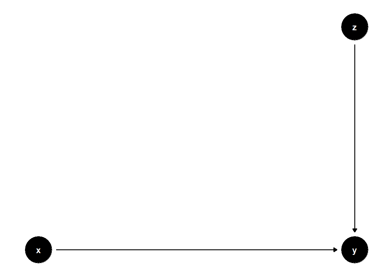

n <- 1e4
z <- rnorm(n)
x <- rnorm(n)
y <- x + 2 * z + rnorm(n)

jtools::export_summs(
  lm(y ~ x),
  lm(y ~ x + z),
  model.names = c("Without Z", "With Predictive Z")
)

	Without Z	With Predictive Z
(Intercept)	-0.01	-0.01
	(0.02)	(0.01)
x	1.01 ***	1.01 ***
	(0.02)	(0.01)
z		2.01 ***
		(0.01)
N	10000	10000
R2	0.17	0.83
*** p < 0.001; ** p < 0.01; * p < 0.05.

The coefficient on $X$ remains unbiased in both models, but standard errors are smaller in the model with $Z$.

39.3.1.2 $Z$ predicts a mediator $M$

rm(list = ls())

model <- dagitty("dag{
  x -> y
  x -> m
  z -> m
  m -> y
}")
coordinates(model) <- list(
  x = c(x = 1, z = 2, m = 2, y = 3),
  y = c(x = 1, z = 2, m = 1, y = 1)
)
ggdag(model) + theme_dag()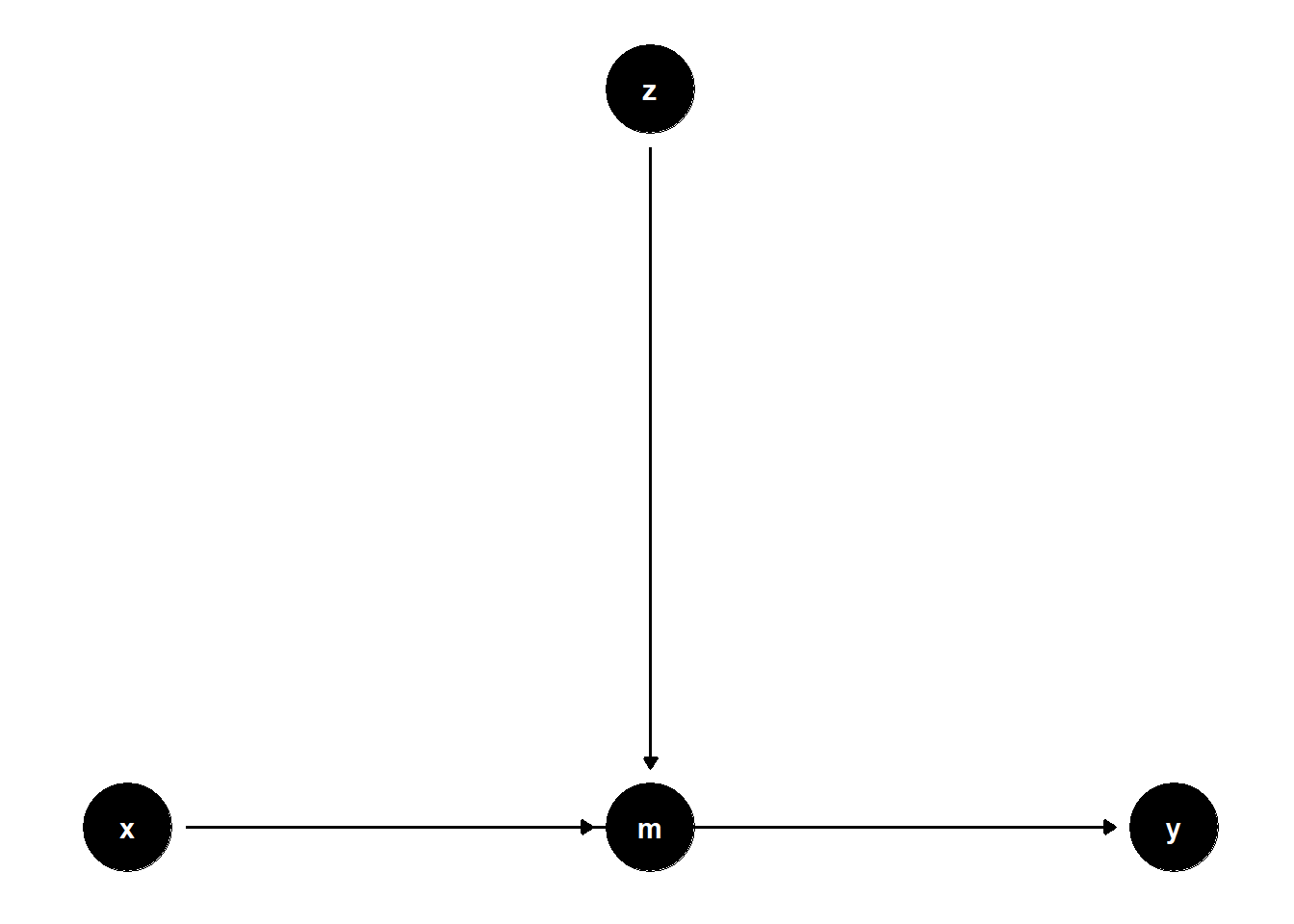

n <- 1e4
z <- rnorm(n)
x <- rnorm(n)
m <- 2 * z + rnorm(n)
y <- x + 2 * m + rnorm(n)

jtools::export_summs(
  lm(y ~ x),
  lm(y ~ x + z),
  model.names = c("Without Z", "With Predictive Z")
)

	Without Z	With Predictive Z
(Intercept)	0.02	0.02
	(0.05)	(0.02)
x	1.04 ***	1.00 ***
	(0.05)	(0.02)
z		3.98 ***
		(0.02)
N	10000	10000
R2	0.05	0.77
*** p < 0.001; ** p < 0.01; * p < 0.05.

Even though $Z$ is not on any causal path from $X$ to $Y$, controlling for it may reduce residual variance in $Y$, hence increasing precision.

39.3.2 Good Selection Bias

In more complex selection structures, adjusting for selection variables can improve identification, but only in the presence of additional post-selection information.

39.3.2.1 $W$ is a collider; $Z$ helps condition on selection

rm(list = ls())

model <- dagitty("dag{
  x -> y
  x -> z
  z -> w
  u -> w
  u -> y
}")
latents(model) <- "u"
coordinates(model) <- list(
  x = c(x = 1, z = 2, w = 3, u = 3, y = 5),
  y = c(x = 3, z = 2, w = 1, u = 4, y = 3)
)
ggdag(model) + theme_dag()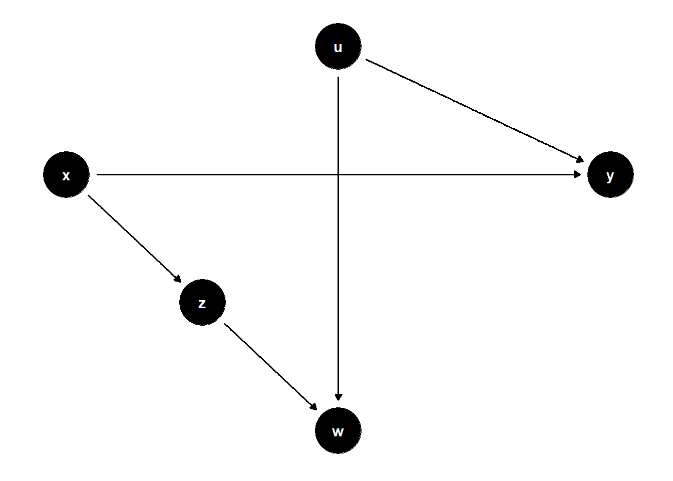

n <- 1e4
x <- rnorm(n)
u <- rnorm(n)
z <- x + rnorm(n)
w <- z + u + rnorm(n)
y <- x - 2 * u + rnorm(n)

jtools::export_summs(
  lm(y ~ x),
  lm(y ~ x + w),
  lm(y ~ x + z + w),
  model.names = c("Unadjusted", "Control W", "Control W + Z")
)

	Unadjusted	Control W	Control W + Z
(Intercept)	-0.00	0.00	-0.02
	(0.02)	(0.02)	(0.02)
x	1.00 ***	1.69 ***	1.01 ***
	(0.02)	(0.02)	(0.02)
w		-0.67 ***	-1.00 ***
		(0.01)	(0.01)
z			1.01 ***
			(0.02)
N	10000	10000	10000
R2	0.18	0.40	0.51
*** p < 0.001; ** p < 0.01; * p < 0.05.

• Unadjusted model is unbiased.

• Controlling only for $W$ is biased due to collider path $X \to Z \to W \leftarrow U \to Y$.

• Adding $Z$ restores identification by blocking that path.

39.3.3 Bad Predictive Controls

Not all predictive variables are useful — some may reduce precision by soaking up degrees of freedom or increasing multicollinearity.

39.3.3.1 $Z$ predicts $X$, not $Y$

rm(list = ls())

model <- dagitty("dag{
  x -> y
  z -> x
}")
coordinates(model) <- list(
  x = c(x = 1, z = 1, y = 2),
  y = c(x = 1, z = 2, y = 1)
)
ggdag(model) + theme_dag()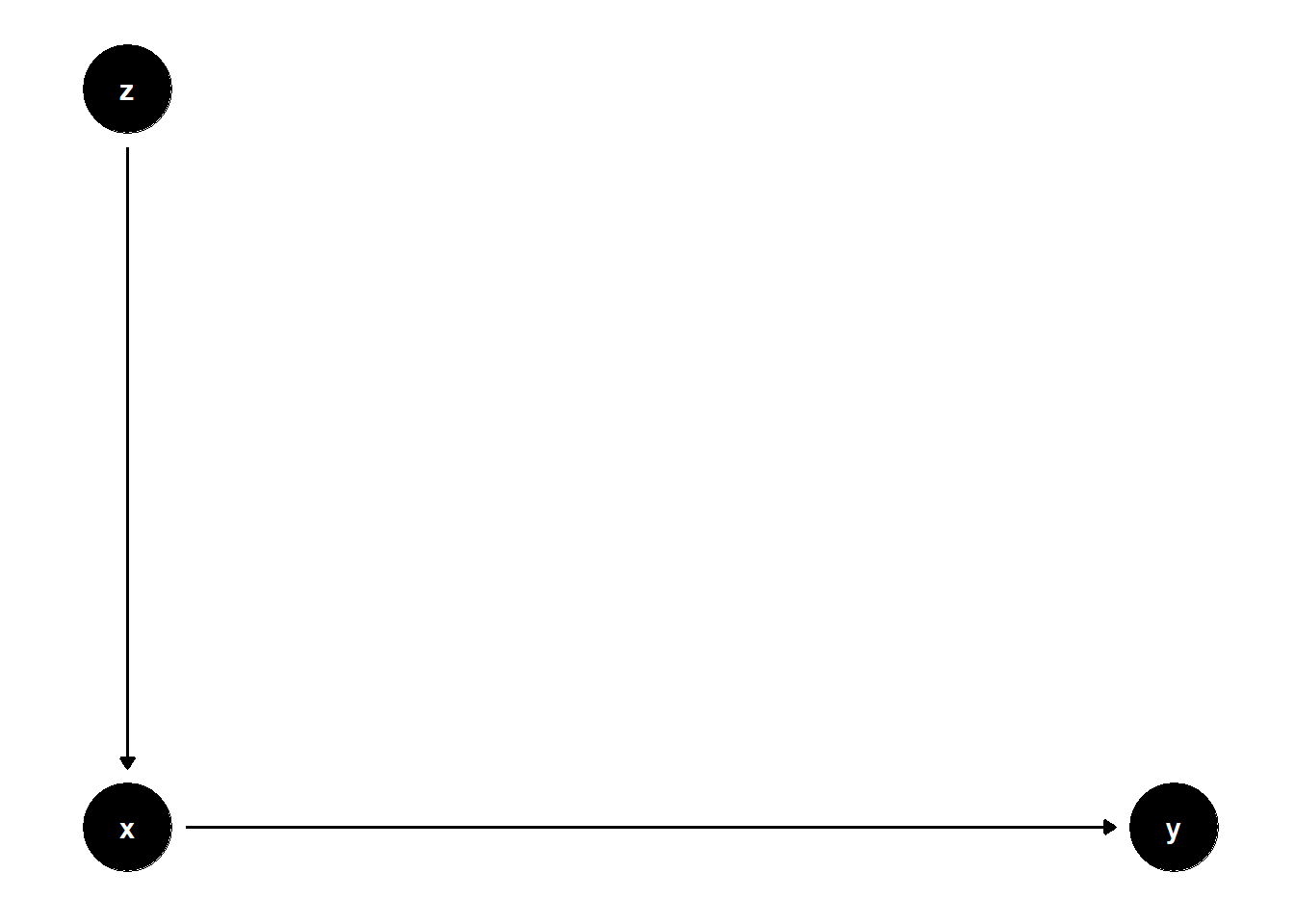

n <- 1e4
z <- rnorm(n)
x <- 2 * z + rnorm(n)
y <- x + rnorm(n)

jtools::export_summs(
  lm(y ~ x),
  lm(y ~ x + z),
  model.names = c("Without Z", "With Z (predicts X)")
)

	Without Z	With Z (predicts X)
(Intercept)	0.01	0.01
	(0.01)	(0.01)
x	1.00 ***	1.00 ***
	(0.00)	(0.01)
z		-0.00
		(0.02)
N	10000	10000
R2	0.84	0.84
*** p < 0.001; ** p < 0.01; * p < 0.05.

$Z$ adds no explanatory power for $Y$, and thus increases SE for the estimate of $X$’s effect.

39.3.3.2 $Z$ is a child of $X$

rm(list = ls())

model <- dagitty("dag{
  x -> y
  x -> z
}")
coordinates(model) <- list(
  x = c(x = 1, z = 1, y = 2),
  y = c(x = 1, z = 2, y = 1)
)
ggdag(model) + theme_dag()

n <- 1e4
x <- rnorm(n)
z <- 2 * x + rnorm(n)
y <- x + rnorm(n)

jtools::export_summs(
  lm(y ~ x),
  lm(y ~ x + z),
  model.names = c("Without Z", "With Child Z")
)

	Without Z	With Child Z
(Intercept)	0.00	0.00
	(0.01)	(0.01)
x	1.02 ***	1.06 ***
	(0.01)	(0.02)
z		-0.02 *
		(0.01)
N	10000	10000
R2	0.49	0.49
*** p < 0.001; ** p < 0.01; * p < 0.05.

Here, $Z$ is a post-treatment variable. Though it does not bias the estimate of $X$, it adds noise and increases the SE.

39.3.4 Bad Selection Bias

Controlling for some post-treatment variables can hurt precision without affecting bias.

rm(list = ls())

model <- dagitty("dag{
  x -> y
  x -> z
}")
coordinates(model) <- list(
  x = c(x = 1, z = 2, y = 2),
  y = c(x = 1, z = 2, y = 1)
)
ggdag(model) + theme_dag()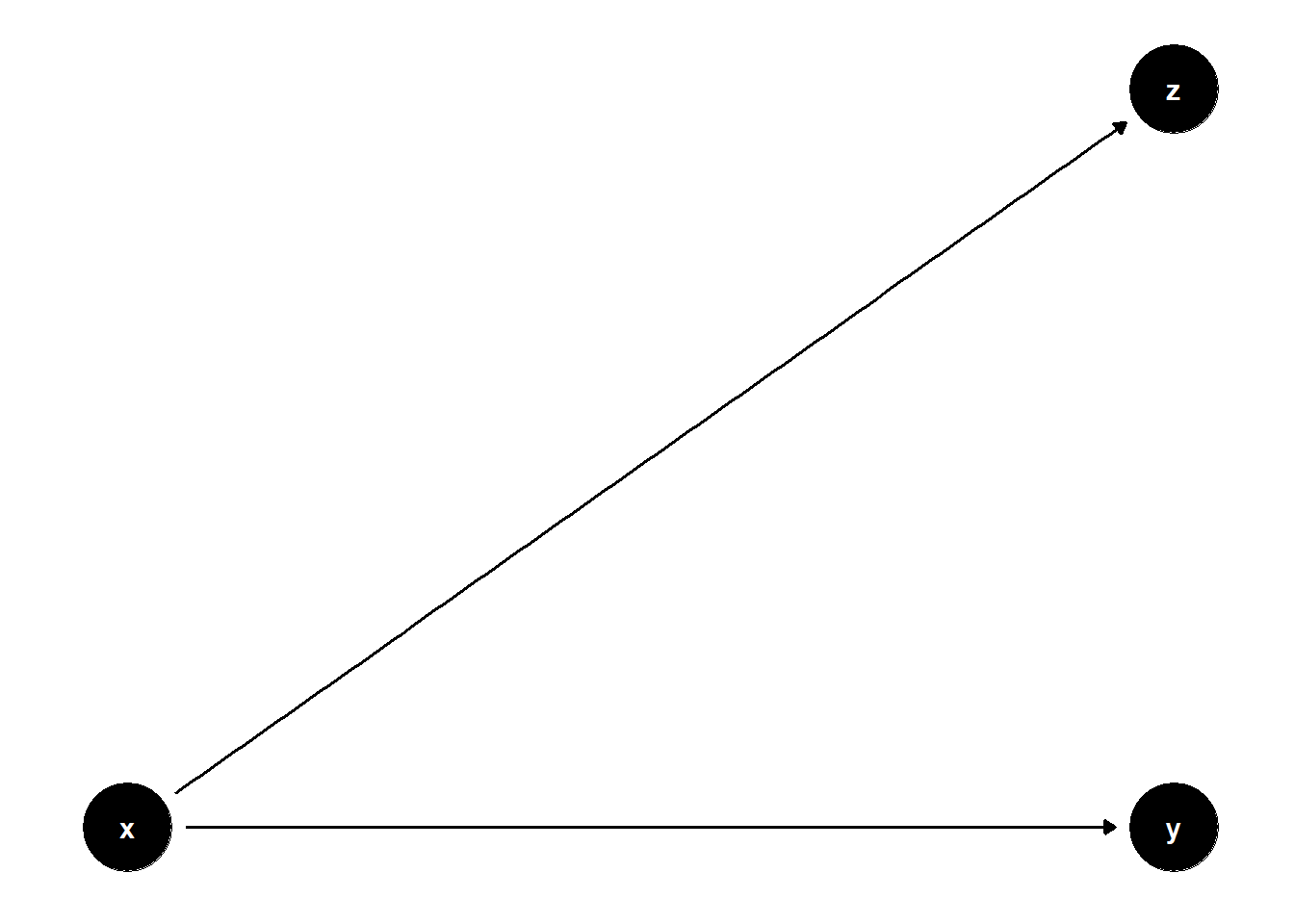

n <- 1e4
x <- rnorm(n)
z <- 2 * x + rnorm(n)
y <- x + rnorm(n)

jtools::export_summs(
  lm(y ~ x),
  lm(y ~ x + z),
  model.names = c("Without Z", "With Post-treatment Z")
)

	Without Z	With Post-treatment Z
(Intercept)	-0.00	-0.00
	(0.01)	(0.01)
x	1.00 ***	0.99 ***
	(0.01)	(0.02)
z		0.01
		(0.01)
N	10000	10000
R2	0.50	0.50
*** p < 0.001; ** p < 0.01; * p < 0.05.

Although $Z$ lies on a causal path from $X$ to $Z$ (and not from $Z$ to $Y$), including $Z$ adds redundant information and may inflate standard errors. In this case, it’s not a “bad control” in the M-bias sense, but still suboptimal.

39.3.5 Summary Table: Predictive vs. Causal Utility of Controls

Control Type	Bias Impact	SE Impact	Causal Use?
Predictive of $Y$, not $X$	None	Improves SE	Optional
Predictive of $X$, not $Y$	None	Hurts SE	Avoid if possible
On causal path ($X \to Z$)	None (if not a mediator)	SE or undercontrol	Avoid unless estimating direct effect
Post-treatment collider	May induce bias	Hurts SE	Avoid
Aids blocking collider paths	May help	Mixed	Conditional

---