33.14 Application of Event Study
Several R packages facilitate event studies. Below are some commonly used ones:
| Package | Description |
|---|---|
eventstudies |
Computes abnormal returns and visualizes event impact |
erer |
Implements event study methodology in economics and finance |
EventStudy |
Provides API-based event study tools (requires subscription) |
AbnormalReturns |
Implements market model and FF3 abnormal return calculations |
PerformanceAnalytics |
Provides tools for risk and performance measurement |
estudy2 |
A flexible event study implementation |
To install these packages, run:
install.packages(
    c(
        "eventstudies",
        "erer",
        "EventStudy",
        "AbnormalReturns",
        "PerformanceAnalytics",
        "tidyquant",
        "tidyverse"
    )
)
33.14.1 Sorting Portfolios for Expected Returns
A common approach in finance is to sort stocks into portfolios based on firm characteristics such as size and book-to-market (B/M) ratio. This method helps control for the possibility that standard models (e.g., Fama-French) may not be correctly specified.
Sorting Process
Sort all stock returns into 10 deciles based on size (market capitalization).
Within each size decile, sort returns into 10 deciles based on B/M ratio.
Calculate the average return of each portfolio for each period (i.e., the expected return for stocks given their characteristics).
Compare each stock’s return to its corresponding portfolio.
Important Notes:
Sorting often leads to more conservative estimates compared to Fama-French models.
If the event study results change depending on the sorting order (e.g., sorting by B/M first vs. size first), this suggests that the findings are not robust.
33.14.2 erer Package
The erer package provides a straightforward implementation of event studies.
Step 1: Load Required Libraries
Step 2: Load Sample Data
The package includes an example dataset, daEsa, which contains stock returns and event dates.
data(daEsa)
head(daEsa)
#>       date       tb3m    sp500     bbc     bow     csk      gp      ip     kmb
#> 1 19900102  0.3973510  1.76420  2.5352  1.3575  0.6289  4.1237  1.3274  1.8707
#> 2 19900103  0.6596306 -0.25889  0.2747  0.8929  6.2500  0.9901 -0.2183 -0.3339
#> 3 19900104 -0.5242464 -0.86503 -1.3699 -0.4425 -2.3529  0.7353 -0.4376 -0.1675
#> 4 19900105 -0.6587615 -0.98041 -0.5556 -0.4444  1.2048  0.0000  0.2198 -0.6711
#> 5 19900108  0.0000000  0.45043 -1.3966 -0.8929 -1.1905  0.4866 -0.2193  1.0135
#> 6 19900109  0.1326260 -1.18567  0.2833 -0.4505 -2.4096 -0.2421 -2.1978 -2.1739
#>       lpx     mwv     pch     pcl      pop     tin     wpp      wy
#> 1  1.7341  1.6529  4.0816  1.5464  2.43525 -1.0791  2.9197  2.7149
#> 2  0.8523  2.0325  0.0000  0.5076  1.41509 -1.4545  0.7092 -2.2026
#> 3 -0.2817  0.3984  0.3268 -0.5051 -0.93023 -0.1845  2.1127 -0.9009
#> 4 -0.8475 -0.3968 -0.6515 -0.5076  0.00000  0.5545 -0.6897 -0.4545
#> 5 -0.5698 -0.3984  0.3279  1.0204 -0.93897 -0.5515 -0.6944  0.0000
#> 6 -0.2865 -1.6000  0.3268 -2.5253 -3.79147 -2.4030  0.6993 -1.8265
Step 3: Compute Abnormal Returns
We define the estimation window (250 days before the event) and the event window (\(\pm5\) days around the event):
hh <- evReturn(
y = daEsa,
firm = "wpp",
y.date = "date",
index = "sp500",
est.win = 250,
event.date = 19990505,
event.win = 5
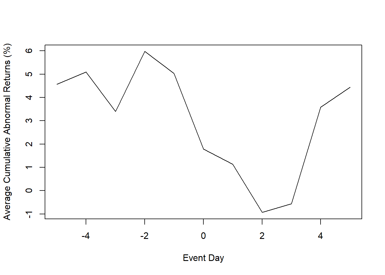
)Step 4: Visualizing the Results
33.14.3 Eventus
2 types of output:
-
Using different estimation methods (e.g., market model to calendar-time approach)
Does not include event-specific returns. Hence, no regression later to determine variables that can affect abnormal stock returns.
Cross-sectional Analysis of Eventus: Event-specific abnormal returns (using monthly or data data) for cross-sectional analysis (under Cross-Sectional Analysis section)
- Since it has the stock-specific abnormal returns, we can do regression on CARs later. But it only gives market-adjusted model. However, according to (A. Sorescu, Warren, and Ertekin 2017), they advocate for the use of market-adjusted model for the short-term only, and reserve the FF4 for the longer-term event studies using monthly daily.
33.14.3.1 Basic Event Study
- Input a text file contains a firm identifier (e.g., PERMNO, CUSIP) and the event date
- Choose market indices: equally weighted and the value weighted index (i.e., weighted by their market capitalization). And check Fama-French and Carhart factors.
- Estimation options
Estimation period:
ESTLEN = 100is the convention so that the estimation is not impacted by outliers.Use “autodate” options: the first trading after the event date is used if the event falls on a weekend or holiday
- Abnormal returns window: depends on the specific event
- Choose test: either parametric (including Patell Standardized Residual (PSR)) or non-parametric
33.14.3.2 Cross-sectional Analysis of Eventus
Similar to the Basic Event Study, but now you can have event-specific abnormal returns.