19.2 Causal Inference Approach to Mediation
Traditional mediation models assume that regression-based estimates provide valid causal inference. However, causal mediation analysis (CMA) extends beyond traditional models by explicitly defining mediation in terms of potential outcomes and counterfactuals.
19.2.1 Example: Traditional Mediation Analysis
We begin with a classic three-step mediation approach.
# Load data
myData <- read.csv("data/mediationData.csv")

# Step 1 (Total Effect: X → Y) [No longer required]
model.0 <- lm(Y ~ X, data = myData)
summary(model.0)
#>
#> Call:
#> lm(formula = Y ~ X, data = myData)
#>
#> Residuals:
#>     Min      1Q  Median      3Q     Max
#> -5.0262 -1.2340 -0.3282  1.5583  5.1622
#>
#> Coefficients:
#>             Estimate Std. Error t value Pr(>|t|)
#> (Intercept)   2.8572     0.6932   4.122 7.88e-05 ***
#> X             0.3961     0.1112   3.564 0.000567 ***
#> ---
#> Signif. codes:  0 '***' 0.001 '**' 0.01 '*' 0.05 '.' 0.1 ' ' 1
#>
#> Residual standard error: 1.929 on 98 degrees of freedom
#> Multiple R-squared:  0.1147, Adjusted R-squared:  0.1057
#> F-statistic:  12.7 on 1 and 98 DF,  p-value: 0.0005671

# Step 2 (Effect of X on M)
model.M <- lm(M ~ X, data = myData)
summary(model.M)
#>
#> Call:
#> lm(formula = M ~ X, data = myData)
#>
#> Residuals:
#>     Min      1Q  Median      3Q     Max
#> -4.3046 -0.8656  0.1344  1.1344  4.6954
#>
#> Coefficients:
#>             Estimate Std. Error t value Pr(>|t|)
#> (Intercept)  1.49952    0.58920   2.545   0.0125 *
#> X            0.56102    0.09448   5.938 4.39e-08 ***
#> ---
#> Signif. codes:  0 '***' 0.001 '**' 0.01 '*' 0.05 '.' 0.1 ' ' 1
#>
#> Residual standard error: 1.639 on 98 degrees of freedom
#> Multiple R-squared:  0.2646, Adjusted R-squared:  0.2571
#> F-statistic: 35.26 on 1 and 98 DF,  p-value: 4.391e-08

# Step 3 (Effect of M on Y, controlling for X)
model.Y <- lm(Y ~ X + M, data = myData)
summary(model.Y)
#>
#> Call:
#> lm(formula = Y ~ X + M, data = myData)
#>
#> Residuals:
#>     Min      1Q  Median      3Q     Max
#> -3.7631 -1.2393  0.0308  1.0832  4.0055
#>
#> Coefficients:
#>             Estimate Std. Error t value Pr(>|t|)
#> (Intercept)   1.9043     0.6055   3.145   0.0022 **
#> X             0.0396     0.1096   0.361   0.7187
#> M             0.6355     0.1005   6.321 7.92e-09 ***
#> ---
#> Signif. codes:  0 '***' 0.001 '**' 0.01 '*' 0.05 '.' 0.1 ' ' 1
#>
#> Residual standard error: 1.631 on 97 degrees of freedom
#> Multiple R-squared:  0.373,  Adjusted R-squared:  0.3601
#> F-statistic: 28.85 on 2 and 97 DF,  p-value: 1.471e-10

# Step 4: Bootstrapping for ACME
library(mediation)
results <-
    mediate(
        model.M,
        model.Y,
        treat = 'X',
        mediator = 'M',
        boot = TRUE,
        sims = 500
    )
summary(results)
#>
#> Causal Mediation Analysis
#>
#> Nonparametric Bootstrap Confidence Intervals with the Percentile Method
#>
#>                 Estimate 95% CI Lower 95% CI Upper p-value
#> ACME            0.356522     0.211871     0.507799  <2e-16 ***
#> ADE             0.039604    -0.174982     0.278427   0.760
#> Total Effect    0.396126     0.174283     0.643540   0.004 **
#> Prop. Mediated  0.900022     0.504160     1.937520   0.004 **
#> ---
#> Signif. codes:  0 '***' 0.001 '**' 0.01 '*' 0.05 '.' 0.1 ' ' 1
#>
#> Sample Size Used: 100
#>
#>
#> Simulations: 500- Total Effect: \(\hat{c} = 0.3961\) → effect of \(X\) on \(Y\) without controlling for \(M\).
- Direct Effect (ADE): \(\hat{c'} = 0.0396\) → effect of \(X\) on \(Y\) after accounting for \(M\).
- ACME (Average Causal Mediation Effect):
ACME = \(\hat{c} - \hat{c'} = 0.3961 - 0.0396 = 0.3565\)
Equivalent to product of paths: \(\hat{a} \times \hat{b} = 0.56102 \times 0.6355 = 0.3565\).
These calculations do not rely on strong causal assumptions. For a causal interpretation, we need a more rigorous framework.
19.2.2 Two Approaches in Causal Mediation Analysis
The mediation package Imai, Keele, and Yamamoto (2010) enables causal mediation analysis. It supports two inference types:
Model-Based Inference
Assumptions:
Treatment is randomized (or approximated via matching).
Sequential Ignorability: No unobserved confounding in:
Treatment → Mediator
Treatment → Outcome
Mediator → Outcome
This assumption is hard to justify in observational studies.
Design-Based Inference
- Relies on experimental design to isolate the causal mechanism.
Notation
We follow the standard potential outcomes framework:
\(M_i(t)\) = mediator under treatment condition \(t\)
\(T_i \in {0,1}\) = treatment assignment
\(Y_i(t, m)\) = outcome under treatment \(t\) and mediator value \(m\)
\(X_i\) = observed pre-treatment covariates
The treatment effect for an individual \(i\): \[ \tau_i = Y_i(1,M_i(1)) - Y_i (0,M_i(0)) \] which decomposes into:
- Causal Mediation Effect (ACME):
\[ \delta_i (t) = Y_i (t,M_i(1)) - Y_i(t,M_i(0)) \]
- Direct Effect (ADE):
\[ \zeta_i (t) = Y_i (1, M_i(1)) - Y_i(0, M_i(0)) \]
Summing up:
\[ \tau_i = \delta_i (t) + \zeta_i (1-t) \]
Sequential Ignorability Assumption
For CMA to be valid, we assume:
\[ \begin{aligned} \{ Y_i (t', m), M_i (t) \} &\perp T_i |X_i = x\\ Y_i(t',m) &\perp M_i(t) | T_i = t, X_i = x \end{aligned} \]
First condition is the standard strong ignorability condition where treatment assignment is random conditional on pre-treatment confounders.
Second condition is stronger where the mediators is also random given the observed treatment and pre-treatment confounders. This condition is satisfied only when there is no unobserved pre-treatment confounders, and post-treatment confounders, and multiple mediators that are correlated.
Key Challenge
Sequential Ignorability is not testable. Researchers should conduct sensitivity analysis.
We now fit a causal mediation model using mediation.
library(mediation)
set.seed(2014)
data("framing", package = "mediation")

# Step 1: Fit mediator model (M ~ T, X)
med.fit <-
    lm(emo ~ treat + age + educ + gender + income, data = framing)

# Step 2: Fit outcome model (Y ~ M, T, X)
out.fit <-
    glm(
        cong_mesg ~ emo + treat + age + educ + gender + income,
        data = framing,
        family = binomial("probit")
    )

# Step 3: Causal Mediation Analysis (Quasi-Bayesian)
med.out <-
    mediate(
        med.fit,
        out.fit,
        treat = "treat",
        mediator = "emo",
        robustSE = TRUE,
        sims = 100
    )  # Use sims = 10000 in practice
summary(med.out)
#>
#> Causal Mediation Analysis
#>
#> Quasi-Bayesian Confidence Intervals
#>
#>                           Estimate 95% CI Lower 95% CI Upper p-value
#> ACME (control)            0.079128     0.035058     0.150095  <2e-16 ***
#> ACME (treated)            0.080385     0.036654     0.155707  <2e-16 ***
#> ADE (control)             0.020551    -0.097597     0.115775    0.70
#> ADE (treated)             0.021808    -0.105256     0.122624    0.70
#> Total Effect              0.100936    -0.049706     0.233869    0.14
#> Prop. Mediated (control)  0.694620    -6.310861     3.679318    0.14
#> Prop. Mediated (treated)  0.711848    -5.793642     3.496550    0.14
#> ACME (average)            0.079756     0.035856     0.153702  <2e-16 ***
#> ADE (average)             0.021180    -0.101427     0.119199    0.70
#> Prop. Mediated (average)  0.703234    -6.052251     3.587934    0.14
#> ---
#> Signif. codes:  0 '***' 0.001 '**' 0.01 '*' 0.05 '.' 0.1 ' ' 1
#>
#> Sample Size Used: 265
#>
#>
#> Simulations: 100
Alternative: Nonparametric Bootstrap
med.out <-
    mediate(
        med.fit,
        out.fit,
        boot = TRUE,
        treat = "treat",
        mediator = "emo",
        sims = 100,
        boot.ci.type = "bca"
    )
summary(med.out)
#>
#> Causal Mediation Analysis
#>
#> Nonparametric Bootstrap Confidence Intervals with the BCa Method
#>
#>                            Estimate 95% CI Lower 95% CI Upper p-value
#> ACME (control)             0.084786     0.042409     0.135927  <2e-16 ***
#> ACME (treated)             0.085820     0.041012     0.136296  <2e-16 ***
#> ADE (control)              0.011654    -0.072556     0.133438    0.58
#> ADE (treated)              0.012689    -0.078400     0.141850    0.58
#> Total Effect               0.097475     0.012219     0.249860    0.06 .
#> Prop. Mediated (control)   0.869822     1.746034   151.198626    0.06 .
#> Prop. Mediated (treated)   0.880437     1.687950   138.906093    0.06 .
#> ACME (average)             0.085303     0.043380     0.137194  <2e-16 ***
#> ADE (average)              0.012172    -0.075578     0.137570    0.58
#> Prop. Mediated (average)   0.875130     1.716992   145.052358    0.06 .
#> ---
#> Signif. codes:  0 '***' 0.001 '**' 0.01 '*' 0.05 '.' 0.1 ' ' 1
#>
#> Sample Size Used: 265
#>
#>
#> Simulations: 100
If we suspect moderation, we include an interaction term.
med.fit <-
    lm(emo ~ treat + age + educ + gender + income, data = framing)

out.fit <-
    glm(
        cong_mesg ~ emo * treat + age + educ + gender + income,
        data = framing,
        family = binomial("probit")
    )

med.out <-
    mediate(
        med.fit,
        out.fit,
        treat = "treat",
        mediator = "emo",
        robustSE = TRUE,
        sims = 100
    )

summary(med.out)
#>
#> Causal Mediation Analysis
#>
#> Quasi-Bayesian Confidence Intervals
#>
#>                             Estimate 95% CI Lower 95% CI Upper p-value
#> ACME (control)             0.0741675    0.0240117    0.1364901  <2e-16 ***
#> ACME (treated)             0.0949636    0.0270237    0.1630112  <2e-16 ***
#> ADE (control)             -0.0135332   -0.1185510    0.1096060    0.76
#> ADE (treated)              0.0072629   -0.1100691    0.1145408    0.90
#> Total Effect               0.0814304   -0.0564589    0.1924589    0.26
#> Prop. Mediated (control)   0.6451040  -14.3124300    3.1336595    0.26
#> Prop. Mediated (treated)   0.9800632  -17.8320223    4.0060277    0.26
#> ACME (average)             0.0845655    0.0273792    0.1470397  <2e-16 ***
#> ADE (average)             -0.0031352   -0.1145684    0.1172708    1.00
#> Prop. Mediated (average)   0.8125836  -16.0722261    3.5478494    0.26
#> ---
#> Signif. codes:  0 '***' 0.001 '**' 0.01 '*' 0.05 '.' 0.1 ' ' 1
#>
#> Sample Size Used: 265
#>
#>
#> Simulations: 100
test.TMint(med.out, conf.level = .95)  # Tests for interaction effect
#>
#>  Test of ACME(1) - ACME(0) = 0
#>
#> data:  estimates from med.out
#> ACME(1) - ACME(0) = 0.020796, p-value = 0.3
#> alternative hypothesis: true ACME(1) - ACME(0) is not equal to 0
#> 95 percent confidence interval:
#>  -0.01757310  0.07110837
Since sequential ignorability is untestable, we examine how unmeasured confounding affects ACME estimates.
# Load required package
library(mediation)

# Simulate some example data
set.seed(123)
n <- 100
data <- data.frame(
  treat = rbinom(n, 1, 0.5),       # Binary treatment
  med = rnorm(n),                   # Continuous mediator
  outcome = rnorm(n)                 # Continuous outcome
)

# Fit the mediator model (med ~ treat)
med_model <- lm(med ~ treat, data = data)

# Fit the outcome model (outcome ~ treat + med)
outcome_model <- lm(outcome ~ treat + med, data = data)

# Perform mediation analysis
med_out <- mediate(med_model,
                   outcome_model,
                   treat = "treat",
                   mediator = "med",
                   sims = 100)

# Conduct sensitivity analysis
sens_out <- medsens(med_out, sims = 100)

summary(sens_out)
#>
#> Mediation Sensitivity Analysis for Average Causal Mediation Effect
#>
#> Sensitivity Region
#>
#>        Rho    ACME 95% CI Lower 95% CI Upper R^2_M*R^2_Y* R^2_M~R^2_Y~
#>  [1,] -0.9 -0.6194      -1.3431       0.1043         0.81       0.7807
#>  [2,] -0.8 -0.3898      -0.8479       0.0682         0.64       0.6168
#>  [3,] -0.7 -0.2790      -0.6096       0.0516         0.49       0.4723
#>  [4,] -0.6 -0.2067      -0.4552       0.0418         0.36       0.3470
#>  [5,] -0.5 -0.1525      -0.3406       0.0355         0.25       0.2409
#>  [6,] -0.4 -0.1083      -0.2487       0.0321         0.16       0.1542
#>  [7,] -0.3 -0.0700      -0.1723       0.0323         0.09       0.0867
#>  [8,] -0.2 -0.0354      -0.1097       0.0389         0.04       0.0386
#>  [9,] -0.1 -0.0028      -0.0648       0.0591         0.01       0.0096
#> [10,]  0.0  0.0287      -0.0416       0.0990         0.00       0.0000
#> [11,]  0.1  0.0603      -0.0333       0.1538         0.01       0.0096
#> [12,]  0.2  0.0928      -0.0317       0.2173         0.04       0.0386
#> [13,]  0.3  0.1275      -0.0333       0.2882         0.09       0.0867
#> [14,]  0.4  0.1657      -0.0369       0.3684         0.16       0.1542
#> [15,]  0.5  0.2100      -0.0422       0.4621         0.25       0.2409
#> [16,]  0.6  0.2642      -0.0495       0.5779         0.36       0.3470
#> [17,]  0.7  0.3364      -0.0601       0.7329         0.49       0.4723
#> [18,]  0.8  0.4473      -0.0771       0.9717         0.64       0.6168
#> [19,]  0.9  0.6768      -0.1135       1.4672         0.81       0.7807
#>
#> Rho at which ACME = 0: -0.1
#> R^2_M*R^2_Y* at which ACME = 0: 0.01
#> R^2_M~R^2_Y~ at which ACME = 0: 0.0096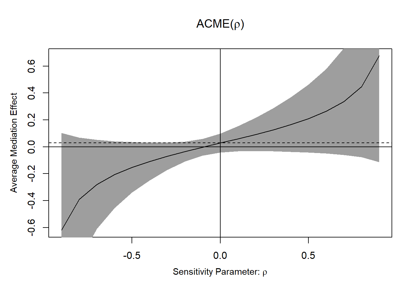
Figure 19.4: ACME
- If ACME confidence intervals contain 0, the effect is not robust to confounding.
Alternatively, using \(R^2\) interpretation, we need to specify the direction of confounder that affects the mediator and outcome variables in plot using sign.prod = "positive" (i.e., same direction) or sign.prod = "negative" (i.e., opposite direction).
| Aspect | Traditional Mediation | Causal Mediation |
|---|---|---|
| Model Assumption | Linear regressions | Potential outcomes framework |
| Assumptions Needed | No omitted confounders | Sequential ignorability |
| Inference Method | Product of coefficients | Counterfactual reasoning |
| Bootstrapping? | Common | Essential |
| Sensitivity Analysis? | Rarely used | Strongly recommended |