21.7 Types of Treatment Effects
When evaluating the causal impact of an intervention, different estimands (quantities of interest) can be used to measure treatment effects, depending on the study design and assumptions about compliance.
Terminology:
- Estimands: The causal effect parameters we seek to measure.
- Estimators: The statistical procedures used to estimate those parameters.
- Sources of Bias (L. Keele and Grieve 2025):
\[ \begin{aligned} &\text{Estimator - True Causal Effect} \\ &= \underbrace{\textbf{Hidden bias}}_{\text{Due to design}} + \underbrace{\textbf{Misspecification bias}}_{\text{Due to modeling}} +\underbrace{\textbf{Statistical noise}}_{\text{Due to finite sample}} \end{aligned} \]
- Hidden Bias (Due to Design)
- Arises from unobserved confounders and measurement error that remain after conditioning on observed covariates.
- Is “hidden” because its true magnitude or direction cannot be directly observed.
- Violations of conditional exchangeability (also called no unobserved confounding) imply the presence of hidden bias.
- Misspecification Bias (Due to Modeling)
- Occurs when the assumed model for the outcome or treatment assignment does not reflect the true data-generating process.
- Persists even if we have perfect exchangeability (i.e., no hidden bias).
- Can be viewed as under-specification (omitting essential terms or functional forms) or over-specification (including unnecessary parameters).
- Statistical Noise (Due to Finite Sample)
- Even with perfect design and correct model specification, finite samples lead to randomness in estimates.
- Standard errors, confidence intervals, and p-values reflect this uncertainty.
In practice, all three sources of bias and uncertainty can coexist to varying degrees.
21.7.1 Average Treatment Effect
The Average Treatment Effect (ATE) is the expected difference in outcomes between individuals who receive treatment and those who do not.
Definition
Let:
\(Y_i(1)\) be the outcome of individual \(i\) under treatment.
\(Y_i(0)\) be the outcome of individual \(i\) under control.
The individual treatment effect is:
\[ \tau_i = Y_i(1) - Y_i(0) \]
Since we cannot observe both \(Y_i(1)\) and \(Y_i(0)\) for the same individual (a fundamental problem in causal inference), we estimate the ATE across a population:
\[ ATE = E[Y(1)] - E[Y(0)] \]
Identification Under Randomization
If treatment assignment is randomized (under Experimental Design), then the observed difference in means between treatment and control groups provides an unbiased estimator of ATE:
\[ ATE = \frac{1}{N} \sum_{i=1}^{N} \tau_i = \frac{\sum_1^N Y_i(1)}{N} - \frac{\sum_i^N Y_i(0)}{N} \]
With randomization, we assume:
\[ E[Y(1) | D = 1] = E[Y(1) | D = 0] = E[Y(1)] \]
\[ E[Y(0) | D = 1] = E[Y(0) | D = 0] = E[Y(0)] \]
Thus, the difference in observed means between treated and control groups provides an unbiased estimate of ATE.
\[ ATE = E[Y(1)] - E[Y(0)] \]
Alternatively, we can express the potential outcomes framework in a regression form, which allows us to connect causal inference concepts with standard regression analysis.
Instead of writing treatment effects as potential outcomes, we can define the observed outcome \(Y_i\) in terms of a regression equation:
\[ Y_i = Y_i(0) + [Y_i (1) - Y_i(0)] D_i \]
where:
\(Y_i(0)\) is the outcome if individual \(i\) does not receive treatment.
\(Y_i(1)\) is the outcome if individual \(i\) does receive treatment.
\(D_i\) is a binary indicator for treatment assignment:
\(D_i = 1\) if individual \(i\) receives treatment.
\(D_i = 0\) if individual \(i\) is in the control group.
We can redefine this equation using regression notation:
\[ Y_i = \beta_{0i} + \beta_{1i} D_i \]
where:
\(\beta_{0i} = Y_i(0)\) represents the baseline (control group) outcome.
\(\beta_{1i} = Y_i(1) - Y_i(0)\) represents the individual treatment effect.
Thus, in an ideal setting, the coefficient on \(D_i\) in a regression gives us the treatment effect.
In observational studies, treatment assignment \(D_i\) is often not random, leading to endogeneity. This means that the error term in the regression equation might be correlated with \(D_i\), violating one of the key assumptions of the Ordinary Least Squares estimator.
To formalize this issue, we can express the outcome equation as:
\[ \begin{aligned} Y_i &= \beta_{0i} + \beta_{1i} D_i \\ &= ( \bar{\beta}_{0} + \epsilon_{0i} ) + (\bar{\beta}_{1} + \epsilon_{1i} )D_i \\ &= \bar{\beta}_{0} + \epsilon_{0i} + \bar{\beta}_{1} D_i + \epsilon_{1i} D_i \end{aligned} \]
where:
\(\bar{\beta}_{0}\) is the average baseline outcome.
\(\bar{\beta}_{1}\) is the average treatment effect.
\(\epsilon_{0i}\) captures individual-specific deviations in control group outcomes.
\(\epsilon_{1i}\) captures heterogeneous treatment effects.
If treatment assignment is truly random, then:
\[ E[\epsilon_{0i}] = E[\epsilon_{1i}] = 0 \]
which ensures:
No selection bias: \(D_i \perp \epsilon_{0i}\) (i.e., treatment assignment is independent of the baseline error).
Treatment effect is independent of assignment: \(D_i \perp \epsilon_{1i}\).
However, in observational studies, these assumptions often fail. This leads to:
- Selection bias: If individuals self-select into treatment based on unobserved characteristics, then \(D_i\) correlates with \(\epsilon_{0i}\).
- Heterogeneous treatment effects: If the treatment effect itself varies across individuals, then \(D_i\) correlates with \(\epsilon_{1i}\).
These issues violate the exogeneity assumption in OLS regression, leading to biased estimates of \(\beta_1\).
When estimating treatment effects using OLS regression, we need to be aware of potential estimation issues.
- OLS Estimator and Difference-in-Means
Under random assignment, the OLS estimator for \(\beta_1\) simplifies to the difference in means estimator:
\[ \hat{\beta}_1^{OLS} = \bar{Y}_{\text{treated}} - \bar{Y}_{\text{control}} \]
which is an unbiased estimator of the Average Treatment Effect.
However, when treatment assignment is not random, OLS estimates may be biased due to unobserved confounders.
- Heteroskedasticity and Robust Standard Errors
If treatment effects vary across individuals (i.e., treatment effect heterogeneity), the error term contains an interaction:
\[ \epsilon_i = \epsilon_{0i} + D_i \epsilon_{1i} \]
which leads to heteroskedasticity (i.e., the variance of errors depends on \(D_i\) and possibly on covariates \(X_i\)).
To address this, we use heteroskedasticity-robust standard errors, which ensure valid inference even when variance is not constant across observations.
21.7.2 Conditional Average Treatment Effect
Treatment effects may vary across different subgroups in a population. The Conditional Average Treatment Effect (CATE) captures heterogeneity in treatment effects across subpopulations.
For a subgroup characterized by covariates \(X_i\):
\[ CATE = E[Y(1) - Y(0) | X_i] \]
Why is CATE Useful?
- Heterogeneous Treatment Effects: Certain groups may benefit more from treatment than others.
- Policy Targeting: Understanding who benefits the most allows for better resource allocation.
Example
- Policy Intervention: A job training program may have different effects on younger vs. older workers.
- Medical Treatments: Drug effectiveness may differ by gender, age, or genetic factors.
Estimating CATE allows policymakers and researchers to identify who benefits most from an intervention.
21.7.3 Intention-to-Treat Effect
A key issue in empirical research is non-compliance, where individuals do not always follow their assigned treatment (i.e., either people who are supposed to receive treatment don’t receive it, or people who are supposed to be in the control group receive the treatment). The Intention-to-Treat (ITT) effect measures the impact of offering treatment, regardless of whether individuals actually receive it.
Definition
The ITT effect is the observed difference in means between groups assigned to treatment and control:
\[ ITT = E[Y | D = 1] - E[Y | D = 0] \]
Why Use ITT?
- Policy Evaluation: ITT reflects the real-world effectiveness of an intervention, accounting for incomplete take-up.
- Randomized Trials: ITT preserves randomization, even when compliance is imperfect.
Example: Vaccination
- A government offers a vaccine (ITT), but not everyone actually takes it.
- The true treatment effect depends on those who receive the vaccine, which differs from the effect measured under ITT.
Since non-compliance is common in real-world settings, ITT effects are often smaller than true treatment effects. In this case, the difference in observed means between the treatment and control groups is not [Average Treatment Effects], but Intention-to-Treat Effect.
21.7.4 Local Average Treatment Effects
In many empirical settings, not all individuals assigned to treatment actually receive it (non-compliance). Instead of estimating the treatment effect for everyone assigned to treatment (i.e., Intention-to-Treat Effects), we often want to estimate the effect of treatment on those who actually comply with their assignment.
This is known as the Local Average Treatment Effect, also referred to as the Complier Average Causal Effect (CACE).
- LATE is the treatment effect for the subgroup of compliers—those who take the treatment if and only if assigned to it.
- Unlike Conditional Average Treatment Effects, which describes heterogeneity across observable subgroups, LATE focuses on compliance behavior.
- We typically recover LATE using Instrumental Variables, leveraging random treatment assignment as an instrument.
21.7.4.1 Estimating LATE Using Instrumental Variables
Instrumental variable estimation allows us to isolate the effect of treatment on compliers by using random treatment assignment as an instrument for actual treatment receipt.
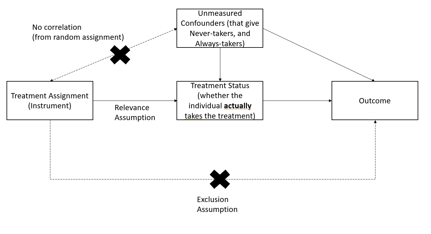
Figure 2.7: LATE Instrumental Variables
From an instrumental variables perspective, LATE is estimated as:
\[ LATE = \frac{ITT}{\text{Share of Compliers}} \]
where:
ITT (Intention-to-Treat Effect) is the effect of being assigned to treatment.
Share of Compliers is the proportion of individuals who actually take the treatment when assigned to it.
21.7.4.2 Key Properties of LATE
- As the proportion of compliers increases, LATE converges to ITT.
- LATE is always larger than ITT, since ITT averages over both compliers and non-compliers.
- Standard error rule of thumb:
The standard error of LATE is given by:
\[ SE(LATE) = \frac{SE(ITT)}{\text{Share of Compliers}} \]
- LATE can also be estimated using a pure placebo group (Gerber et al. 2010).
- Partial compliance is difficult to study
- The IV/2SLS estimator is biased in small samples, requiring Bayesian methods for correction (Long, Little, and Lin 2010; Jin and Rubin 2009, 2008).
21.7.4.3 One-Sided Noncompliance
One-sided noncompliance occurs when we observe only compliers and never-takers in the sample (i.e., no always-takers).
Key assumptions:
Exclusion Restriction (Excludability): Never-takers have the same outcomes regardless of assignment (i.e., treatment has no effect on them because they never receive it).
Random Assignment Ensures Balance: The number of never-takers is expected to be equal in the treatment and control groups.
Estimation of LATE under one-sided noncompliance:
\[ LATE = \frac{ITT}{\text{Share of Compliers}} \]
Since the never-takers do not receive treatment, this simplifies estimation.
21.7.4.4 Two-Sided Noncompliance
Two-sided noncompliance occurs when we observe compliers, never-takers, and always-takers in the sample.
Key assumptions:
Exclusion Restriction (Excludability): Never-takers and always-takers have the same outcome regardless of treatment assignment.
Monotonicity Assumption (No Defiers):
There are no defiers, meaning no individuals systematically avoid treatment when assigned to it.
This assumption is standard in practical studies.
Estimation of LATE under two-sided noncompliance:
\[ LATE = \frac{ITT}{\text{Share of Compliers}} \]
- Since always-takers receive treatment regardless of assignment, their presence does not bias LATE as long as monotonicity holds.
- In practice, monotonicity is often reasonable, as defiers are rare.
| Scenario | What it Measures | When to Use It? | Key Assumptions |
|---|---|---|---|
| Intention-to-Treat | Effect of being assigned to treatment | Policy impact with non-compliance | None (preserves randomization) |
| LATE | Effect on compliers only | When we care about actual treatment effect rather than assignment | Excludability, Monotonicity (No Defiers) |
21.7.5 Population vs. Sample Average Treatment Effects
In experimental and observational studies, we often estimate the Sample Average Treatment Effect (SATE) using a finite sample. However, the Population Average Treatment Effect (PATE) is the parameter of interest when making broader generalizations.
Key Issue:
SATE does not necessarily equal PATE due to sample selection bias and treatment imbalance.
See (Imai, King, and Stuart 2008) for an in-depth discussion on when SATE diverges from PATE.
Consider a finite population of size \(N\) from which we observe a sample of size \(n\) (\(N \gg n\)). Half of the sample receives treatment, and half is assigned to control.
Define the following indicators:
Sampling Indicator:
\[ I_i = \begin{cases} 1, & \text{if unit } i \text{ is in the sample} \\ 0, & \text{otherwise} \end{cases} \]Treatment Assignment Indicator:
\[ T_i = \begin{cases} 1, & \text{if unit } i \text{ is in the treatment group} \\ 0, & \text{if unit } i \text{ is in the control group} \end{cases} \]Potential Outcomes Framework:
\[ Y_i = \begin{cases} Y_i(1), & \text{if } T_i = 1 \text{ (Treated)} \\ Y_i(0), & \text{if } T_i = 0 \text{ (Control)} \end{cases} \]Observed Outcome:
Since we can never observe both potential outcomes for the same unit, the observed outcome is:\[ Y_i | I_i = 1 = T_i Y_i(1) + (1 - T_i) Y_i(0) \]
True Individual Treatment Effect:
The individual-level treatment effect is:\[ TE_i = Y_i(1) - Y_i(0) \]
However, since we observe only one of \(Y_i(1)\) or \(Y_i(0)\), \(TE_i\) is never directly observed.
21.7.5.1 Definitions of SATE and PATE
Sample Average Treatment Effect (SATE): \[ SATE = \frac{1}{n} \sum_{i \in \{I_i = 1\}} TE_i \] SATE is the average treatment effect within the sample.
Population Average Treatment Effect (PATE): \[ PATE = \frac{1}{N} \sum_{i=1}^N TE_i \] PATE represents the true treatment effect across the entire population.
Since we observe only a subset of the population, SATE may not equal PATE.
21.7.5.2 Decomposing Estimation Error
The baseline estimator for SATE and PATE is the difference in observed means:
\[ \begin{aligned} D &= \frac{1}{n/2} \sum_{i \in (I_i = 1, T_i = 1)} Y_i - \frac{1}{n/2} \sum_{i \in (I_i = 1 , T_i = 0)} Y_i \\ &= \text{(Mean of Treated Group)} - \text{(Mean of Control Group)} \end{aligned} \]
Define \(\Delta\) as the estimation error (i.e., deviation from the truth), under an additive model:
\[ Y_i(t) = g_t(X_i) + h_t(U_i) \]
The estimation error is decomposed into
\[ \begin{aligned} PATE - D = \Delta &= \Delta_S + \Delta_T \\ &= (PATE - SATE) + (SATE - D)\\ &= \text{Sample Selection Bias} + \text{Treatment Imbalance} \\ &= (\Delta_{S_X} + \Delta_{S_U}) + (\Delta_{T_X} + \Delta_{T_U}) \\ &= (\text{Selection on Observables} + \text{Selection on Unobservables}) \\ &+ (\text{Treatment Imbalance in Observables} + \text{Treatment Imbalance in Unobservables}) \end{aligned} \]
To further illustrate this, we begin by explicitly defining how the total discrepancy \(PATE - D\) separates into different components.
Step 1: From \(PATE - D\) to \(\Delta_S + \Delta_T\)
\[ \underbrace{PATE - D}_{\Delta} = \underbrace{(PATE - SATE)}_{\Delta_S} + \underbrace{(SATE - D)}_{\Delta_T}. \]
- \(PATE - D\): The total discrepancy between the true population treatment effect and the estimate \(D\).
- \(\Delta_S = PATE - SATE\): Sample Selection Bias – how much the sample ATE differs from the population ATE.
- \(\Delta_T = SATE - D\): Treatment Imbalance – how much the estimated treatment effect deviates from the sample ATE.
Step 2: Breaking Bias into Observables and Unobservables
Each bias term can be decomposed into observed (\(X\)) and unobserved (\(U\)) factors:
\[ \Delta_S = \underbrace{\Delta_{S_X}}_{\text{Selection on Observables}} + \underbrace{\Delta_{S_U}}_{\text{Selection on Unobservables}} \]
\[ \Delta_T = \underbrace{\Delta_{T_X}}_{\text{Treatment Imbalance in Observables}} + \underbrace{\Delta_{T_U}}_{\text{Treatment Imbalance in Unobservables}} \]
Thus, the final expression:
\[ \begin{aligned} PATE - D &= \underbrace{(PATE - SATE)}_{\Delta_S:\text{Sample Selection Bias}} + \underbrace{(SATE - D)}_{\Delta_T:\text{Treatment Imbalance}} \\ &= \underbrace{(\Delta_{S_X} + \Delta_{S_U})}_{\text{Selection on }X + \text{ Selection on }U} + \underbrace{(\Delta_{T_X} + \Delta_{T_U})}_{\text{Imbalance in }X + \text{ Imbalance in }U}. \end{aligned} \]
This decomposition clarifies the sources of error in estimating the true effect, distinguishing between sample representativeness (selection bias) and treatment assignment differences (treatment imbalance), and further separating these into observable and unobservable components.
21.7.5.2.1 Sample Selection Bias ( \(\Delta_S\) )
Also called sample selection error, this arises when the sample is not representative of the population.
\[ \Delta_S = PATE - SATE = \frac{N - n}{N}(NATE - SATE) \]
where:
- NATE (Non-Sample Average Treatment Effect) is the average treatment effect for the part of the population not included in the sample:
\[ NATE = \sum_{i\in (I_i = 0)} \frac{TE_i}{N-n} \]
To eliminate sample selection bias (\(\Delta_S = 0\)):
- Redefine the sample as the entire population (\(N = n\)).
- Ensure \(NATE = SATE\) (e.g., treatment effects must be homogeneous across sampled and non-sampled units).
However, when treatment effects vary across individuals, random sampling only warrants sample selection bias but does not sample eliminate error.
21.7.5.2.2 Treatment Imbalance Error ( \(\Delta_T\) )
Also called treatment imbalance bias, this occurs when the empirical distribution of treated and control units differs.
\[ \Delta_T = SATE - D \]
Key insight:
\(\Delta_T \to 0\) when the treatment and control groups are balanced across both observables (\(X\)) and unobservables (\(U\)).
Since we cannot directly adjust for unobservables, imbalance correction methods focus on observables.
21.7.5.3 Adjusting for (Observable) Treatment Imbalance
However, in real-world studies:
We can only adjust for observables \(X\), not unobservables \(U\).
Residual imbalance in unobservables may still introduce bias after adjustment.
To address treatment imbalance, researchers commonly use:
| Method | Blocking | Matching Methods |
|---|---|---|
| Definition | Random assignment within predefined strata based on pre-treatment covariates. | Dropping, repeating, or grouping observations to balance covariates between treated and control groups (Rubin 1973). |
| When Applied? | Before treatment assignment (in experimental designs). | After treatment assignment (in observational studies). |
| Effectiveness | Ensures exact balance within strata but may require large sample sizes for fine stratification. | Can improve balance, but risk of increasing bias if covariates are poorly chosen. |
| What If Covariates Are Irrelevant? | No effect on treatment estimates. | Worst-case scenario: If matching is done on covariates uncorrelated with treatment but correlated with outcomes, it may increase bias instead of reducing it. |
| Benefits | Eliminates imbalance in observables (\(\Delta_{T_X} = 0\)). Effect on unobservables is uncertain (may help if unobservables correlate with observables). |
Reduces model dependence, bias, variance, and mean-squared error (MSE). Matching only balances observables, and its effect on unobservables is unknown. |
21.7.6 Average Treatment Effects on the Treated and Control
In many empirical studies, researchers are interested in how treatment affects specific subpopulations rather than the entire population. Two commonly used treatment effect measures are:
- Average Treatment Effect on the Treated (ATT): The effect of treatment on individuals who actually received treatment.
- Average Treatment Effect on the Control (ATC): The effect treatment would have had on individuals who were not treated.
Understanding the distinction between ATT, ATC, and ATE is crucial for determining external validity and for designing targeted policies.
21.7.6.1 Average Treatment Effect on the Treated
The ATT measures the expected treatment effect only for those who were actually treated:
\[ \begin{aligned} ATT &= E[Y_i(1) - Y_i(0) | D_i = 1] \\ &= E[Y_i(1) | D_i = 1] - E[Y_i(0) | D_i = 1] \end{aligned} \]
Key Interpretation:
ATT tells us how much better (or worse) off treated individuals are compared to their hypothetical counterfactual outcome (had they not been treated).
It is useful for evaluating the effectiveness of interventions on those who self-select into treatment.
21.7.6.2 Average Treatment Effect on the Control
The ATC measures the expected treatment effect only for those who were not treated:
\[ \begin{aligned} ATC &= E[Y_i(1) - Y_i(0) | D_i = 0] \\ &= E[Y_i(1) | D_i = 0] - E[Y_i(0) | D_i = 0] \end{aligned} \]
Key Interpretation:
ATC answers the question: “What would have been the effect of treatment if it had been given to those who were not treated?”
It is important for understanding how an intervention might generalize to untreated populations.
21.7.6.3 Relationship Between ATT, ATC, and ATE
Under random assignment and full compliance, we have:
\[ ATE = ATT = ATC \]
Why?
Randomization ensures that treated and untreated groups are statistically identical before treatment.
Thus, treatment effects are the same across groups, leading to ATT = ATC = ATE.
However, in observational settings, selection bias and treatment heterogeneity may cause ATT and ATC to diverge from ATE.
21.7.6.4 Sample Average Treatment Effect on the Treated
The Sample ATT (SATT) is the empirical estimate of ATT in a finite sample:
\[ SATT = \frac{1}{n} \sum_{i \in D_i = 1} TE_i \]
where:
\(TE_i = Y_i(1) - Y_i(0)\) is the treatment effect for unit \(i\).
\(n\) is the number of treated units in the sample.
The summation is taken only over treated units in the sample.
21.7.6.5 Population Average Treatment Effect on the Treated
The Population ATT (PATT) generalizes ATT to the entire treated population:
\[ PATT = \frac{1}{N} \sum_{i \in D_i = 1} TE_i \]
where:
\(TE_i = Y_i(1) - Y_i(0)\) is the treatment effect for unit \(i\).
\(N\) is the total number of treated units in the population.
The summation is taken over all treated individuals in the population.
If the sample is randomly drawn, then \(SATT \approx PATT\), but if the sample is not representative, \(SATT\) may overestimate or underestimate \(PATT\).
21.7.6.6 When ATT and ATC Diverge from ATE
In real-world studies, ATT and ATC often differ from ATE due to treatment effect heterogeneity and selection bias.
21.7.6.6.1 Selection Bias in ATT
If individuals self-select into treatment, then the treated group may be systematically different from the control group.
- Example:
- Suppose a job training program is voluntary.
- Individuals who enroll might be more motivated or have better skills than those who do not.
- As a result, the treatment effect (ATT) may not generalize to the untreated group (ATC).
This implies:
\[ ATT \neq ATC \]
unless treatment assignment is random.
21.7.6.6.2 Treatment Effect Heterogeneity
If treatment effects vary across individuals, then:
- ATT may be larger or smaller than ATE, depending on how treatment effects differ across subgroups.
- ATC may be larger or smaller than ATT, if the untreated group would have responded differently to treatment.
Example:
A scholarship program may be more beneficial for students from lower-income families than for students from wealthier backgrounds.
If lower-income students are more likely to apply for the scholarship, then ATT > ATE.
However, if wealthier students (who did not receive the scholarship) would have benefited less from it, then ATC < ATE.
Thus, we may observe:
\[ ATE \neq ATT \neq ATC \]
| Treatment Effect | Definition | Use Case | Potential Issues |
|---|---|---|---|
| ATE (Average Treatment Effect) | Effect on randomly selected individuals | Policy decisions applicable to entire population | Requires full randomization |
| ATT (Average Treatment on Treated) | Effect on those who received treatment | Evaluating effectiveness of interventions for targeted groups | Selection bias if treatment is voluntary |
| ATC (Average Treatment on Control) | Effect if treatment were given to untreated individuals | Predicting treatment effects for new populations | May not be generalizable |
21.7.7 Quantile Average Treatment Effects
Instead of focusing on the mean effect (ATE), Quantile Treatment Effects (QTE) help us understand how treatment shifts the entire distribution of an outcome variable.
The Quantile Treatment Effect at quantile \(\tau\) is defined as:
\[ QTE_{\tau} = Q_{\tau} (Y_1) - Q_{\tau} (Y_0) \]
where:
\(Q_{\tau} (Y_1)\) is the \(\tau\)-th quantile of the outcome distribution under treatment.
\(Q_{\tau} (Y_0)\) is the \(\tau\)-th quantile of the outcome distribution under control.
When to Use QTE?
- Heterogeneous Treatment Effects: If treatment effects differ across individuals, ATE may be misleading.
- Policy Targeting: Policymakers may care more about low-income individuals (e.g., bottom 25%) rather than the average effect.
- Distributional Changes: QTE allows us to assess whether treatment increases inequality (e.g., benefits the rich more than the poor).
Estimation of QTE
QTE can be estimated using:
Quantile Regression: Extends linear regression to estimate effects at different quantiles.
Instrumental Variables for QTE: Requires additional assumptions to estimate causal effects in the presence of endogeneity (Abadie, Angrist, and Imbens 2002; Chernozhukov and Hansen 2005).
Example: Wage Policy Impact
- Suppose a minimum wage increase is introduced.
- The ATE might show a small positive effect on earnings.
- However, QTE might reveal:
- No effect at the bottom quantiles (for workers who lose jobs).
- A positive effect at the median.
- A strong positive effect at the top quantiles (for experienced workers who benefit the most).
Thus, QTE provides a more detailed view of the treatment effect across the entire income distribution.
21.7.8 Log-Odds Treatment Effects for Binary Outcomes
When the outcome variable is binary (e.g., success/failure, employed/unemployed, survived/died), it is often useful to measure the treatment effect in log-odds form.
For a binary outcome \(Y\), define the probability of success as:
\[ P(Y = 1 | D = d) \]
The log-odds of success under treatment and control are:
\[ \text{Log-odds}(Y | D = 1) = \log \left( \frac{P(Y = 1 | D = 1)}{1 - P(Y = 1 | D = 1)} \right) \]
\[ \text{Log-odds}(Y | D = 0) = \log \left( \frac{P(Y = 1 | D = 0)}{1 - P(Y = 1 | D = 0)} \right) \]
The Log-Odds Treatment Effect (LOTE) is then:
\[ LOTE = \text{Log-odds}(Y | D = 1) - \text{Log-odds}(Y | D = 0) \]
This captures how treatment affects the relative likelihood of success in a nonlinear way.
When to Use Log-Odds Treatment Effects?
- Binary Outcomes: When the treatment outcome is 0 or 1 (e.g., employed/unemployed).
- Nonlinear Treatment Effects: Log-odds help handle situations where effects are multiplicative rather than additive.
- Rare Events: Useful in cases where the outcome probability is very small or very large.
Estimation of Log-Odds Treatment Effects
Logistic Regression with Treatment Indicator: \[ \log \left( \frac{P(Y = 1 | D = 1)}{1 - P(Y = 1 | D = 1)} \right) = \beta_0 + \beta_1 D \] where \(\beta_1\) represents the log-odds treatment effect.
Randomization-Based Estimation: Freedman (2008) provides a framework for randomized trials that ensures consistent estimation.
Attributable Effects: Alternative methods, such as those in (Rosenbaum 2002), estimate the proportion of cases attributable to the treatment.
21.7.9 Summary Table: Treatment Effect Estimands
| Treatment Effect | Definition | Use Case | Key Assumptions | When It Differs from ATE? |
|---|---|---|---|---|
| Average Treatment Effect | The expected treatment effect for a randomly chosen individual in the population. | General policy evaluation; measures the overall impact. | Randomization or strong ignorability (treatment assignment independent of potential outcomes). | - |
| Conditional Average Treatment Effect | The treatment effect for a specific subgroup of the population, conditional on covariates \(X\). | Identifies heterogeneous effects; useful for targeted interventions. | Treatment effect heterogeneity must exist. | Differs when treatment effects vary across subgroups. |
| Intention-to-Treat Effect | The effect of being assigned to treatment, regardless of actual compliance. | Policy evaluations where non-compliance exists. | Randomized treatment assignment ensures unbiased estimation. | Lower than ATE when not all assigned individuals comply. |
| Local Average Treatment Effect | The effect of treatment only on compliers—those who take the treatment if and only if assigned to it. | When compliance is imperfect, LATE isolates the effect for compliers. | Monotonicity (no defiers); instrument only affects the outcome through treatment. | Differs from ATE when compliance is selective. |
| Average Treatment Effect on the Treated | The effect of treatment on those who actually received the treatment. | Used when assessing effectiveness of a treatment for those who self-select into it. | No unmeasured confounders within the treated group. | Differs when treatment selection is not random. |
| Average Treatment Effect on the Control | The effect the treatment would have had on individuals who were not treated. | Predicts the effect of expanding a program to the untreated population. | No unmeasured confounders within the control group. | Differs when treatment effects are heterogeneous. |
| Sample Average Treatment Effect | The estimated treatment effect in the sample. | Used when evaluating treatment within a specific sample. | Sample must be representative of the population for external validity. | Differs when the sample is not representative of the population. |
| Population Average Treatment Effect | The expected treatment effect for the entire population. | Policy design and large-scale decision-making. | Requires that sample selection is random. | Differs when sample selection bias exists. |
| Quantile Treatment Effect | The treatment effect at a specific percentile of the outcome distribution. | Understanding distributional effects rather than mean effects. | Rank preservation or monotonicity assumptions may be needed. | Differs when treatment effects vary across outcome quantiles. |
| Log-Odds Treatment Effect | The effect of treatment on binary outcomes, expressed in log-odds. | Used when outcomes are dichotomous (e.g., employed/unemployed, survived/died). | Logistic model assumptions must hold. | Differs when treatment effects are nonlinear or outcome probabilities are low. |