6.3 Practical Considerations
For optimization algorithms to converge, they require good initial estimates of the parameters. The choice of starting values, constraints, and the complexity of the model all play a role in whether an optimization algorithm successfully finds a suitable solution.
6.3.1 Selecting Starting Values
Choosing good starting values can significantly impact the efficiency and success of optimization algorithms. Several approaches can be used:
- Prior or theoretical information: If prior knowledge about the parameters is available, it should be incorporated into the choice of initial values.
- Grid search or graphical inspection of \(SSE(\theta)\): Evaluating the sum of squared errors (SSE) across a grid of possible values can help identify promising starting points.
- Ordinary Least Squares estimates: If a linear approximation of the model exists, using OLS to obtain initial estimates can be effective.
- Model interpretation: Understanding the structure and behavior of the model can provide intuition for reasonable starting values.
- Expected Value Parameterization: Reformulating the model based on expected values may improve the interpretability and numerical stability of the estimation.
6.3.1.1 Grid Search for Optimal Starting Values
# Set seed for reproducibility
set.seed(123)

# Generate x as 100 integers using seq function
x <- seq(0, 100, 1)

# Generate coefficients for exponential function
a <- runif(1, 0, 20)  # Random coefficient a
b <- runif(1, 0.005, 0.075)  # Random coefficient b
c <- runif(101, 0, 5)  # Random noise

# Generate y as a * e^(b*x) + c
y <- a * exp(b * x) + c

# Print the generated parameters
cat("Generated coefficients:\n")
#> Generated coefficients:
cat("a =", a, "\n")
#> a = 5.75155
cat("b =", b, "\n")
#> b = 0.06018136

# Define our data frame
datf <- data.frame(x, y)

# Define our model function
mod <- function(a, b, x) {
  a * exp(b * x)
}
# Ensure all y values are positive (avoid log issues)
y_adj <-
ifelse(y > 0, y, min(y[y > 0]) + 1e-3) # Shift small values slightly
# Create adjusted dataframe
datf_adj <- data.frame(x, y_adj)
# Linearize by taking log(y)
lin_mod <- lm(log(y_adj) ~ x, data = datf_adj)
# Extract starting values
astrt <-
exp(coef(lin_mod)[1]) # Convert intercept back from log scale
bstrt <- coef(lin_mod)[2] # Slope remains the same
cat("Starting values for non-linear fit:\n")
print(c(astrt, bstrt))
# Fit nonlinear model with these starting values
nlin_mod <- nls(y ~ mod(a, b, x),
start = list(a = astrt, b = bstrt),
data = datf)
# Model summary
summary(nlin_mod)
# Plot original data
plot(
x,
y,
main = "Exponential Growth Fit",
col = "blue",
pch = 16,
xlab = "x",
ylab = "y"
)
# Add fitted curve in red
lines(x, predict(nlin_mod), col = "red", lwd = 2)
# Add legend
legend(
"topleft",
legend = c("Original Data", "Fitted Model"),
col = c("blue", "red"),
pch = c(16, NA),
lwd = c(NA, 2)
)# Define grid of possible parameter values
aseq <- seq(10, 18, 0.2)
bseq <- seq(0.001, 0.075, 0.001)
na <- length(aseq)
nb <- length(bseq)
SSout <- matrix(0, na * nb, 3) # Matrix to store SSE values
cnt <- 0
# Evaluate SSE across grid
for (k in 1:na) {
for (j in 1:nb) {
cnt <- cnt + 1
ypred <-
# Evaluate model at these parameter values
mod(aseq[k], bseq[j], x)
# Compute SSE
ss <- sum((y - ypred) ^ 2)
SSout[cnt, 1] <- aseq[k]
SSout[cnt, 2] <- bseq[j]
SSout[cnt, 3] <- ss
}
}
# Identify optimal starting values
mn_indx <- which.min(SSout[, 3])
astrt <- SSout[mn_indx, 1]
bstrt <- SSout[mn_indx, 2]
# Fit nonlinear model using optimal starting values
nlin_modG <-
nls(y ~ mod(a, b, x), start = list(a = astrt, b = bstrt))
# Display model results
summary(nlin_modG)
#>
#> Formula: y ~ mod(a, b, x)
#>
#> Parameters:
#> Estimate Std. Error t value Pr(>|t|)
#> a 5.889e+00 1.986e-02 296.6 <2e-16 ***
#> b 5.995e-02 3.644e-05 1645.0 <2e-16 ***
#> ---
#> Signif. codes: 0 '***' 0.001 '**' 0.01 '*' 0.05 '.' 0.1 ' ' 1
#>
#> Residual standard error: 2.135 on 99 degrees of freedom
#>
#> Number of iterations to convergence: 4
#> Achieved convergence tolerance: 7.213e-06Note: The nls_multstart package can perform a grid search more efficiently without requiring manual looping.
Visualizing Prediction Intervals
Once the model is fitted, it is useful to visualize prediction intervals to assess model uncertainty.
# Load necessary package
library(nlstools)

# Plot fitted model with confidence and prediction intervals
investr::plotFit(
  nlin_modG,
  interval = "both",
  pch = 19,
  shade = TRUE,
  col.conf = "skyblue4",
  col.pred = "lightskyblue2",
  data = datf
)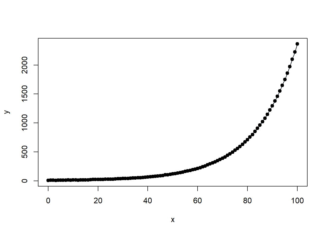
Figure 6.24: Exponential Growth Fit
6.3.1.2 Using Programmed Starting Values in nls
Many nonlinear models have well-established functional forms, allowing for programmed starting values in the nls function. For example, models such as logistic growth and asymptotic regression have built-in self-starting functions.
To explore available self-starting models in R, use:
This command lists functions with names starting with SS, which typically denote self-starting functions for nonlinear regression.
6.3.1.3 Custom Self-Starting Functions
If your model does not match any built-in nls functions, you can define your own self-starting function. Self-starting functions in R automate the process of estimating initial values, which helps in fitting nonlinear models more efficiently.
If needed, a self-starting function should:
Define the nonlinear equation.
Implement a method for computing starting values.
Return the function structure in an appropriate format.
6.3.2 Handling Constrained Parameters
In some cases, parameters must satisfy constraints (e.g., \(\theta_i > a\) or \(a < \theta_i < b\)). The following strategies help address constrained parameter estimation:
- Fit the model without constraints first: If the unconstrained parameter estimates satisfy the desired constraints, no further action is needed.
- Re-parameterization: If the estimated parameters violate constraints, consider re-parameterizing the model to naturally enforce the required bounds.
6.3.3 Failure to Converge
Several factors can cause an algorithm to fail to converge:
- A “flat” SSE function: If the sum of squared errors \(SSE(\theta)\) is relatively constant in the neighborhood of the minimum, the algorithm may struggle to locate an optimal solution.
- Poor starting values: Trying different or better initial values can help.
- Overly complex models: If the model is too complex relative to the data, consider simplifying it.
6.3.4 Convergence to a Local Minimum
- Linear least squares models have a well-defined, unique minimum because the SSE function is quadratic:
\[ SSE(\theta) = (Y - X\beta)'(Y - X\beta) \] - Nonlinear least squares models may have multiple local minima.
- Testing different starting values can help identify a global minimum.
- Graphing \(SSE(\theta)\) as a function of individual parameters (if feasible) can provide insights.
- Alternative optimization algorithms such as Genetic Algorithm or particle swarm optimization may be useful in non-convex problems.
6.3.5 Model Adequacy and Estimation Considerations
Assessing the adequacy of a nonlinear model involves checking its nonlinearity, goodness of fit, and residual behavior. Unlike linear models, nonlinear models do not always have a direct equivalent of \(R^2\), and issues such as collinearity, leverage, and residual heteroscedasticity must be carefully evaluated.
6.3.5.1 Components of Nonlinearity
D. M. Bates and Watts (1980) defines two key aspects of nonlinearity in statistical modeling:
- Intrinsic Nonlinearity
- Measures the bending and twisting in the function \(f(\theta)\).
- Assumes that the function is relatively flat (planar) in the neighborhood of \(\hat{\theta}\).
- If severe, the distribution of residuals will be distorted.
- Leads to:
- Slow convergence of optimization algorithms.
- Difficulties in identifying parameter estimates.
- Solution approaches:
- Higher-order Taylor expansions for estimation.
- Bayesian methods for parameter estimation.
library(MASS)

# Check intrinsic curvature
modD <- deriv3(~ a * exp(b * x), c("a", "b"), function(a, b, x) NULL)

nlin_modD <- nls(y ~ modD(a, b, x),
                 start = list(a = astrt, b = bstrt),
                 data = datf)

rms.curv(nlin_modD)  # Function from the MASS package to assess curvature
#> Parameter effects: c^theta x sqrt(F) = 0.0564
#> Intrinsic: c^iota x sqrt(F) = 9e-04- Parameter-Effects Nonlinearity
Measures how the curvature (nonlinearity) depends on the parameterization.
Strong parameter effects nonlinearity can cause problems with inference on \(\hat{\theta}\).
Can be assessed using:
rms.curvfunction fromMASS.Bootstrap-based inference.
Solution: Try reparameterization to stabilize the function.
6.3.5.2 Goodness of Fit in Nonlinear Models
In linear regression, we use the standard coefficient of determination ($R^2$):
\[ R^2 = \frac{SSR}{SSTO} = 1 - \frac{SSE}{SSTO} \]where:
\(SSR\) = Regression Sum of Squares
\(SSE\) = Error Sum of Squares
\(SSTO\) = Total Sum of Squares
However, in nonlinear models, the error and model sum of squares do not necessarily add up to the total corrected sum of squares:
\[ SSR + SSE \neq SST \]
Thus, \(R^2\) is not directly valid in the nonlinear case. Instead, we use a pseudo-\(R^2\):
\[ R^2_{pseudo} = 1 - \frac{\sum_{i=1}^n ({Y}_i- \hat{Y})^2}{\sum_{i=1}^n (Y_i- \bar{Y})^2} \]
Unlike true \(R^2\), this cannot be interpreted as the proportion of variability explained by the model.
Should be used only for relative model comparison (e.g., comparing different nonlinear models).
6.3.5.3 Residual Analysis in Nonlinear Models
Residual plots help assess model adequacy, particularly when intrinsic curvature is small.
In nonlinear models, the studentized residuals are:
\[ r_i = \frac{e_i}{s \sqrt{1-\hat{c}_i}} \]
where:
\(e_i\) = residual for observation \(i\)
\(\hat{c}_i\) = \(i\)th diagonal element of the tangent-plane hat matrix:
\[ \mathbf{\hat{H} = F(\hat{\theta})[F(\hat{\theta})'F(\hat{\theta})]^{-1}F(\hat{\theta})'} \]
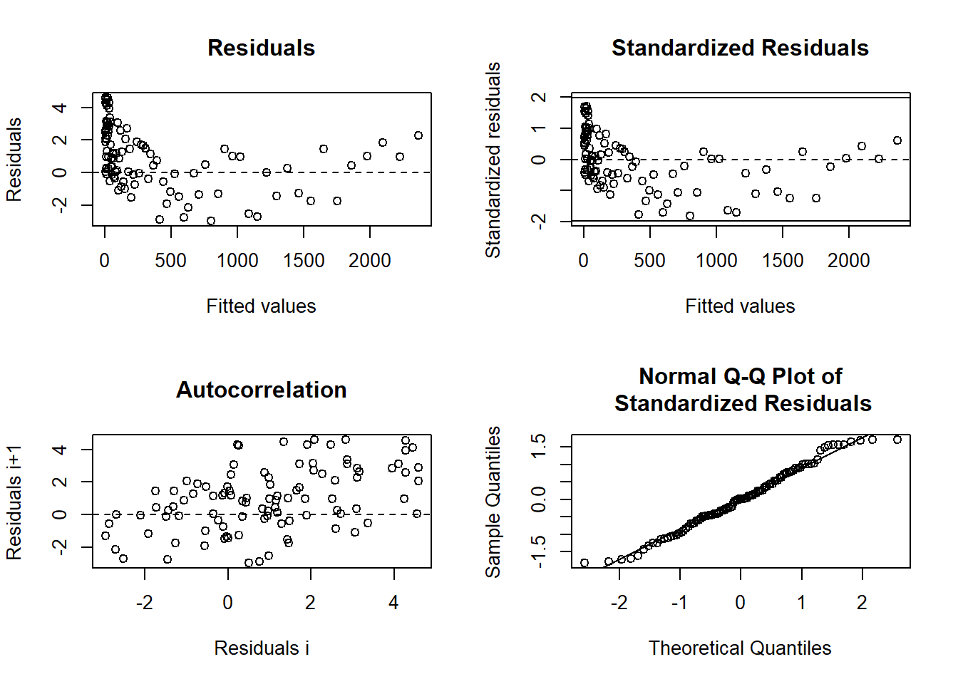
Figure 6.25: Diagnostic Plots for Regression Residuals
6.3.5.4 Potential Issues in Nonlinear Regression Models
6.3.5.4.1 Collinearity
Measures how correlated the model’s predictors are.
In nonlinear models, collinearity is assessed using the condition number of:
\[ \mathbf{[F(\hat{\theta})'F(\hat{\theta})]^{-1}} \]
If condition number > 30, collinearity is a concern.
Solution: Consider reparameterization (Magel and Hertsgaard 1987).
6.3.5.4.2 Leverage
Similar to leverage in Ordinary Least Squares.
In nonlinear models, leverage is assessed using the tangent-plane hat matrix:
\[ \mathbf{\hat{H} = F(\hat{\theta})[F(\hat{\theta})'F(\hat{\theta})]^{-1}F(\hat{\theta})'} \]
- Solution: Identify influential points and assess their impact on parameter estimates (St Laurent and Cook 1992).