30.11 Assumptions
- Parallel Trends Assumption
The Difference-in-Differences estimator relies on a key identifying assumption: the parallel trends assumption. This assumption states that, in the absence of treatment, the average outcome for the treated group would have evolved over time in the same way as for the control group.
Let:
\(Y_{it}(0)\) denote the potential outcome without treatment for unit \(i\) at time \(t\)
\(D_i = 1\) if unit \(i\) is in the treatment group, and \(D_i = 0\) if in the control group
Then, the parallel trends assumption can be written as:
\[ E[Y_{it}(0) \mid D_i = 1] - E[Y_{it}(0) \mid D_i = 0] = \Delta_0 \quad \text{for all } t, \]
where \(\Delta_0\) is a constant difference over time in the untreated potential outcomes between the two groups. This assumption does not require the levels of outcomes to be the same between groups, only that the difference remains constant over time.
In other words, the gap between treatment and control groups in the absence of treatment must remain stable. If this holds, any deviation from that stable difference after the treatment is attributed to the causal effect of the treatment.
It is important to understand how the parallel trends assumption compares to other, stronger assumptions:
Same untreated levels across groups:
A stronger assumption would require that the treated and control groups have identical untreated outcomes at all times:\[ E[Y_{it}(0) \mid D_i = 1] = E[Y_{it}(0) \mid D_i = 0] \quad \text{for all } t \]
This is often unrealistic in observational settings, where baseline characteristics typically differ between groups.
No change in untreated outcomes over time:
Another strong assumption is that untreated outcomes remain constant over time, for both groups:\[ E[Y_{it}(0)] = E[Y_{i,t'}(0)] \quad \text{for all } i \text{ and times } t, t' \]
This implies no secular trends, which is rarely plausible in real-world applications where outcomes (e.g., sales, earnings, health metrics) naturally evolve over time.
The parallel trends assumption is weaker than both of these and is generally more defensible, especially when supported by pre-treatment data.
DiD is appropriate when:
You have pre-treatment and post-treatment outcome data
You have clearly defined treatment and control groups
The parallel trends assumption is plausible
Avoid using DiD when:
Treatment assignment is not random or quasi-random
Unobserved confounders may cause the groups to evolve differently over time
Testing Parallel Trends: Prior Parallel Trends Test.
- No Anticipation Effect (Pre-Treatment Exogeneity)
Individuals or groups should not change their behavior before the treatment is implemented in expectation of the treatment.
If units anticipate the treatment and adjust their behavior beforehand, it can introduce bias in the estimates.
- Exogenous Treatment Assignment
- Treatment should not be assigned based on potential outcomes.
- Ideally, assignment should be as good as random, conditional on observables.
- Stable Composition of Groups (No Attrition or Spillover)
- Treatment and control groups should remain stable over time.
- There should be no selective attrition (where individuals enter/leave due to treatment).
- No spillover effects: Control units should not be indirectly affected by treatment.
- No Simultaneous Confounding Events (Exogeneity of Shocks)
- There should be no other major shocks that affect treatment/control groups differently at the same time as treatment implementation.
- Random Sampling (or Representative Sampling)
Assumption: The units (e.g., individuals, firms, regions) in the treatment and control groups are drawn from the same population, or at least from populations that would follow parallel trends in the absence of treatment.
Implication: Ensures external validity. It allows the DID estimator to generalize to the population of interest and prevents selection bias that would arise if treated and control units were systematically different at baseline.
- Overlap (also called Common Support)
Assumption: There is a positive probability of being treated or untreated for all units. Formally, for any covariate profile, there must be both treated and control units.
Implication: Without overlap, it becomes impossible to construct a valid counterfactual for some treated units. This assumption is especially important in staggered or generalized DID settings where treatment timing varies.
Diagnostic: One can assess this assumption using propensity score distributions or visualizations (e.g., covariate balance plots).
- Effect Additivity (also called Constant Treatment Effect or Additive Structure or Effect Homogeneity)
Assumption: The treatment effect is additive and homogeneous across units and time, meaning that the treatment only shifts the outcome level, not its trend or curvature. In the simplest form: \(Y_{it}(1) - Y_{it}(0) = \delta\) for all \(i\),\(t\)
Implication: This assumption is not required for identification per se, but it simplifies estimation and interpretation. Violations may bias estimates if treatment effects vary in ways that interact with time or unit characteristics.
Alternative Approaches: More recent DID methods (e.g., Callaway & Sant’Anna, Sun & Abraham) relax this assumption by allowing treatment effect heterogeneity.
In a standard DID setup, researchers often use the phrases “effect additivity” and “effect homogeneity” interchangeably, because the customary linear-in-levels model embeds both ideas. Strictly speaking, however, they are not identical (Table 30.8).
| Concept | What it literally requires | What it rules out | Relationship |
|---|---|---|---|
| Effect Additivity | Treated potential outcome equals untreated potential outcome plus a constant shift: \(Y_{it}(1)=Y_{it}(0)+\tau\). The treatment enters the outcome additively and the size of the shift does not depend on the baseline level of the outcome. | Any multiplicative or nonlinear functional form of the effect (e.g., a constant percentage change). | Implies a constant level effect. Guarantees homogeneity and linearity. |
| Effect Homogeneity | The treatment effect \(\tau\) is constant across units and periods: \(\tau_i=\tau_t=\tau\). It says nothing about whether that constant is added, multiplied, or otherwise applied. | Unit-specific or time-varying treatment effects. | A broader statement. You can have homogeneous multiplicative effects (\(Y_{it}(1)=Y_{it}(0)\times\lambda\) with constant \(\lambda\)). Those satisfy homogeneity but violate additivity. |
Why they get conflated in practice
Linear DID regression in levels.
The canonical two-way fixed-effects model, \(Y_{it}= \alpha_i+\lambda_t+\tau D_{it}+\varepsilon_{it}\) identifies \(\tau\) only if (a) the effect is additive and (b) the constant \(\tau\) is the same for every \(i\), \(t\). Hence both additivity and homogeneity are baked in; many textbooks label the joint restriction simply “homogeneous treatment effects”Terminology drift.
Recent heterogeneity papers contrast “TWFE with homogeneous effects” against “heterogeneous effects” without separating additivity from constancy, so the two terms are often treated as synonyms even though, conceptually, homogeneity could hold on another scale.
Practical implications
If you keep the outcome in levels, invoking homogeneous treatment effects effectively commits you to additivity as well.
If the outcome is log-transformed, homogeneous effects correspond to a constant percentage change, which is multiplicative, so additivity no longer holds.
Robustness exercises that re-estimate the model in logs, differences, or growth rates test sensitivity to the additivity choice; stability across scales supports the idea that it is the constancy, not the functional form, that drives the results.
30.11.1 Prior Parallel Trends Test
The parallel trends assumption ensures that, absent treatment, the treated and control groups would have followed similar outcome trajectories. Testing this assumption involves visualization and statistical analysis.
Marcus and Sant’Anna (2021) discuss pre-trend testing in staggered DiD.
- Visual Inspection: Outcome Trends and Treatment Rollout
- Plot raw outcome trends for both groups before and after treatment.
- Use event-study plots to check for pre-trend violations and anticipation effects.
- Visualization tools like
ggplot2orpanelViewhelp illustrate treatment timing and trends.
- Event-Study Regressions
A formal test for pre-trends uses the event-study model:
\[ Y_{it} = \alpha + \sum_{k=-K}^{K} \beta_k 1(T = k) + X_{it} \gamma + \lambda_i + \delta_t + \epsilon_{it} \]
where:
\(1(T = k)\) are time dummies for periods before and after treatment.
\(\beta_k\) captures deviations in outcomes before treatment; these should be statistically indistinguishable from zero if parallel trends hold.
\(\lambda_i\) and \(\delta_t\) are unit and time fixed effects.
\(X_{it}\) are optional covariates.
Violation of parallel trends occurs if pre-treatment coefficients (\(\beta_k\) for \(k < 0\)) are statistically significant.
- Statistical Test for Pre-Treatment Trend Differences
Using only pre-treatment data, estimate:
\[ Y = \alpha_g + \beta_1 T + \beta_2 (T \times G) + \epsilon \]
where:
\(\beta_2\) measures differences in time trends between groups.
If \(\beta_2 = 0\), trends are parallel before treatment.
Considerations:
- Alternative functional forms (e.g., polynomials or nonlinear trends) can be tested.
- If \(\beta_2 \neq 0\), potential explanations include:
- Large sample size driving statistical significance.
- Small deviations in one period disrupting an otherwise stable trend.
While time fixed effects can partially address violations of parallel trends (and are commonly used in modern research), they may also absorb part of the treatment effect, especially when treatment effects vary over time (Wolfers 2003).
Debate on Parallel Trends
- Levels vs. Trends: Kahn-Lang and Lang (2020) argue that similarity in levels is also crucial. If treatment and control groups start at different levels, why assume their trends will be the same?
- Solution:
- Plot time series for the treated and control groups.
- Use matched samples to improve comparability (Ryan et al. 2019) (useful when parallel trends assumption is questionable).
- If levels differ significantly, functional form assumptions become more critical and must be justified.
- Solution:
- Power of Pre-Trend Tests:
- Pre-trend tests often lack statistical power, making false negatives common (Roth 2022).
- See: PretrendsPower and pretrends (for adjustments).
- Outcome Transformations Matter:
- The parallel trends assumption is specific to both the transformation and units of the outcome variable (Roth and Sant’Anna 2023).
- Conduct falsification tests to check whether the assumption holds under different functional forms.
library(tidyverse)
library(fixest)
od <- causaldata::organ_donations %>%
    # Use only pre-treatment data
    filter(Quarter_Num <= 3) %>%
    # Treatment variable
    dplyr::mutate(California = State == 'California')
# use my package
causalverse::plot_par_trends(
data = od,
metrics_and_names = list("Rate" = "Rate"),
treatment_status_var = "California",
time_var = list(Quarter_Num = "Time"),
display_CI = F
)
#> [[1]]
Figure 30.23: Parallel Trends for Rate
# do it manually
# always good but plot the dependent out
od |>
    # group by treatment status and time
    dplyr::group_by(California, Quarter) |>
    dplyr::summarize_all(mean) |>
    dplyr::ungroup() |>
    # view()

    ggplot2::ggplot(aes(x = Quarter_Num, y = Rate, color = California)) +
    ggplot2::geom_line() +
    causalverse::ama_theme()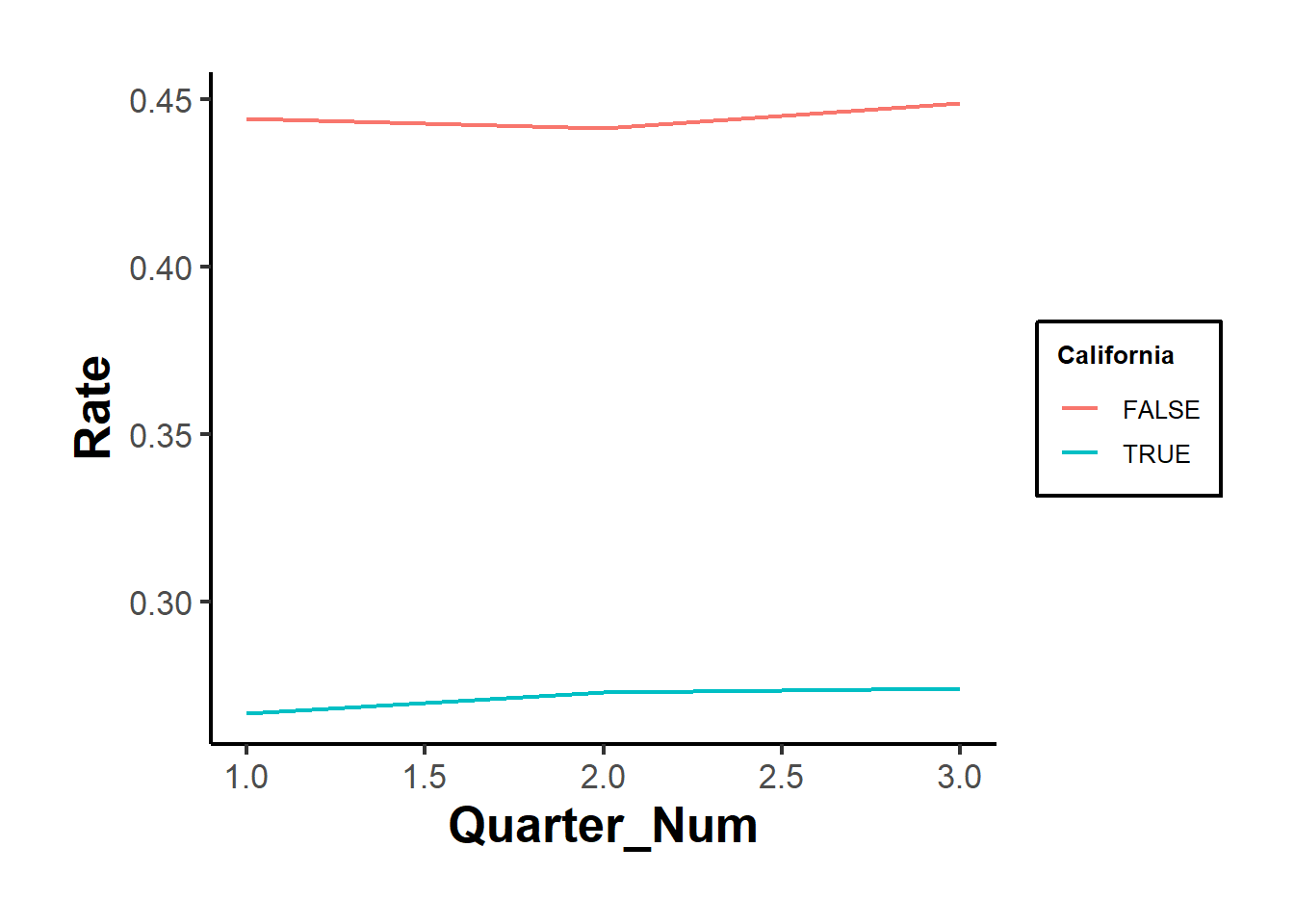
Figure 30.24: Manual parallel trends plot showing average rates
Figures 30.23 and 30.24 show the raw outcomes by periods, while Figure 30.25 shows their coefficient estimates’ version.
# but it's also important to use statistical test
prior_trend <- fixest::feols(Rate ~ i(Quarter_Num, California) |
                                 State + Quarter,
                             data = od)

fixest::coefplot(prior_trend, grid = F)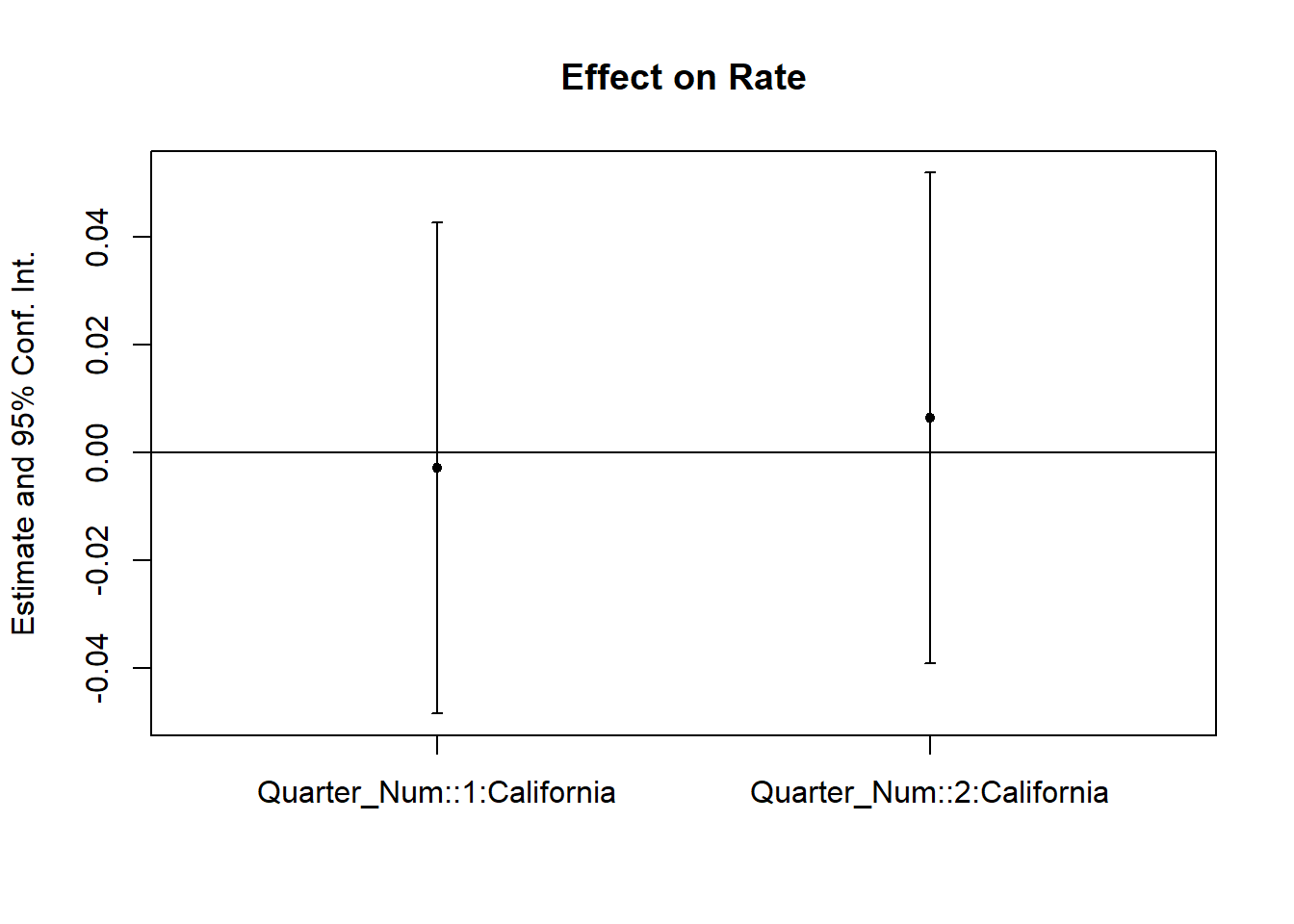
Figure 30.25: Coefficient plot for prior trend analysis
If one of the periods is significantly different from 0, our parallel trends assumption is not plausible.
In cases where the parallel trends assumption is questionable, researchers should consider methods for assessing and addressing potential violations. Some key approaches are discussed in Rambachan and Roth (2023):
Imposing Restrictions: Constrain how different the post-treatment violations of parallel trends can be relative to pre-treatment deviations.
Partial Identification: Rather than assuming a single causal effect, derive bounds on the ATT.
Sensitivity Analysis: Evaluate how sensitive the results are to potential deviations from parallel trends.
To implement these approaches, the HonestDiD package by Rambachan and Roth (2023) provides robust statistical tools:
# https://github.com/asheshrambachan/HonestDiD
# remotes::install_github("asheshrambachan/HonestDiD")
# library(HonestDiD)
Alternatively, Ban and Kedagni (2022) propose a method that incorporates pre-treatment covariates as an information set and makes an assumption about the selection bias in the post-treatment period. Specifically, they assume that the selection bias lies within the convex hull of all pre-treatment selection biases. Under this assumption:
They identify a set of possible ATT values.
With a stronger assumption on selection bias, grounded in policymakers’ perspectives, they can estimate a point estimate of ATT.
Another useful tool for assessing parallel trends is the pretrends package by Roth (2022), which provides formal pre-trend tests:
30.11.2 Placebo Test
A placebo test is a diagnostic tool used in Difference-in-Differences analysis to assess whether the estimated treatment effect is driven by pre-existing trends rather than the treatment itself. The idea is to estimate a treatment effect in a scenario where no actual treatment occurred. If a significant effect is found, it suggests that the parallel trends assumption may not hold, casting doubt on the validity of the causal inference.
Types of Placebo DiD Tests
- Group-Based Placebo Test
- Assign treatment to a group that was never actually treated and rerun the DiD model.
- If the estimated treatment effect is statistically significant, this suggests that differences between groups, not the treatment, are driving results.
- This test helps rule out the possibility that the estimated effect is an artifact of unobserved systematic differences.
A valid treatment effect should be consistent across different reasonable control groups. To assess this:
Rerun the DiD model using an alternative but comparable control group.
Compare the estimated treatment effects across multiple control groups.
If results vary significantly, this suggests that the choice of control group may be influencing the estimated effect, indicating potential selection bias or unobserved confounding.
- Time-Based Placebo Test
- Conduct DiD using only pre-treatment data, pretending that treatment occurred at an earlier period.
- A significant estimated treatment effect implies that differences in pre-existing trends, not treatment, are responsible for observed post-treatment effects.
- This test is particularly useful when concerns exist about unobserved shocks or anticipatory effects.
Random Reassignment of Treatment
- Keep the same treatment and control periods but randomly assign treatment to units that were not actually treated.
- If a significant DiD effect still emerges, it suggests the presence of biases, unobserved confounding, or systematic differences between groups that violate the parallel trends assumption.
Procedure for a Placebo Test
- Using Pre-Treatment Data Only
A robust placebo test often involves analyzing only pre-treatment periods to check whether spurious treatment effects appear. The procedure includes:
Restricting the sample to pre-treatment periods only.
Assigning a fake treatment period before the actual intervention.
Testing a sequence of placebo cutoffs over time to examine whether different assumed treatment timings yield significant effects.
Generating random treatment periods and using randomization inference to assess the sampling distribution of the placebo effect.
Estimating the DiD model using the fake post-treatment period (
post_time = 1).Interpretation: If the estimated treatment effect is statistically significant, this indicates that pre-existing trends (not treatment) might be influencing results, violating the parallel trends assumption.
- Using Control Groups for a Placebo Test
If multiple control groups are available, a placebo test can also be conducted by:
Dropping the actual treated group from the analysis.
Assigning one of the control groups as a fake treated group.
Estimating the DiD model and checking whether a significant effect is detected.
Interpretation:
If a placebo effect appears (i.e., the estimated treatment effect is significant), it suggests that even among control groups, systematic differences exist over time.
However, this result is not necessarily disqualifying. Some methods, such as Synthetic Control, explicitly model such differences while maintaining credibility.
# Load necessary libraries
library(tidyverse)
library(fixest)
library(ggplot2)
library(causaldata)

# Load the dataset
od <- causaldata::organ_donations %>%
    # Use only pre-treatment data
    dplyr::filter(Quarter_Num <= 3) %>%

    # Create fake (placebo) treatment variables
    dplyr::mutate(
        FakeTreat1 = as.integer(State == 'California' &
                                    Quarter %in% c('Q12011', 'Q22011')),
        FakeTreat2 = as.integer(State == 'California' &
                                    Quarter == 'Q22011')
    )

# Estimate the placebo effects using fixed effects regression
clfe1 <- fixest::feols(Rate ~ FakeTreat1 | State + Quarter, data = od)
clfe2 <- fixest::feols(Rate ~ FakeTreat2 | State + Quarter, data = od)

# Display the regression results
fixest::etable(clfe1, clfe2)
#>                           clfe1            clfe2
#> Dependent Var.:            Rate             Rate
#>
#> FakeTreat1      0.0061 (0.0195)
#> FakeTreat2                      -0.0017 (0.0195)
#> Fixed-Effects:  --------------- ----------------
#> State                       Yes              Yes
#> Quarter                     Yes              Yes
#> _______________ _______________ ________________
#> S.E. type                   IID              IID
#> Observations                 81               81
#> R2                      0.99377          0.99376
#> Within R2               0.00192          0.00015
#> ---
#> Signif. codes: 0 '***' 0.001 '**' 0.01 '*' 0.05 '.' 0.1 ' ' 1

# Extract coefficients and confidence intervals
coef_df <- tibble(
    Model = c("FakeTreat1", "FakeTreat2"),
    Estimate = c(coef(clfe1)["FakeTreat1"], coef(clfe2)["FakeTreat2"]),
    SE = c(summary(clfe1)$coeftable["FakeTreat1", "Std. Error"],
           summary(clfe2)$coeftable["FakeTreat2", "Std. Error"]),
    Lower = Estimate - 1.96 * SE,
    Upper = Estimate + 1.96 * SE
)
# Plot the placebo effects
ggplot(coef_df, aes(x = Model, y = Estimate)) +
geom_point(size = 3, color = "blue") +
geom_errorbar(aes(ymin = Lower, ymax = Upper), width = 0.2, color = "blue") +
geom_hline(yintercept = 0, linetype = "dashed", color = "red") +
theme_minimal() +
labs(
title = "Placebo Treatment Effects",
y = "Estimated Effect on Organ Donation Rate",
x = "Placebo Treatment"
)
Figure 30.26: Placebo treatment effects on organ donation rate
We would like the “supposed” DiD to be insignificant (Figure 30.26).