13.3 Diagnosing the Missing Data Mechanism
Understanding the mechanism behind missing data is critical to choosing the appropriate methods for handling it. The three main mechanisms for missing data are MCAR (Missing Completely at Random), MAR (Missing at Random), and MNAR (Missing Not at Random). This section discusses methods for diagnosing these mechanisms, including descriptive and inferential approaches.
13.3.1 Descriptive Methods
13.3.1.1 Visualizing Missing Data Patterns
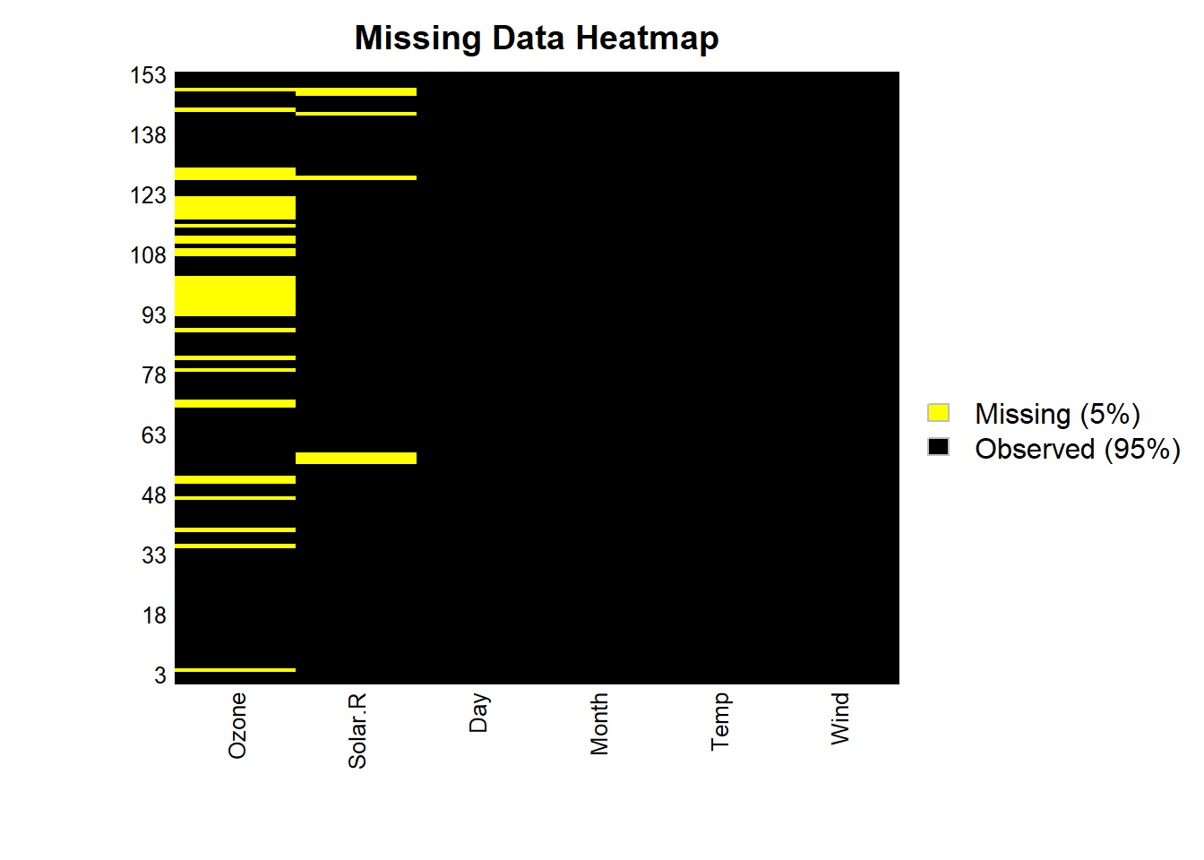
Visualization tools are essential for detecting patterns in missing data. Heatmaps and correlation plots can help identify systematic missingness and provide insights into the underlying mechanism.
# Example: Visualizing missing data
library(Amelia)
missmap(
    airquality,
    main = "Missing Data Heatmap",
    col = c("yellow", "black"),
    legend = TRUE
)
Figure 13.1: Missing Data Heatmap
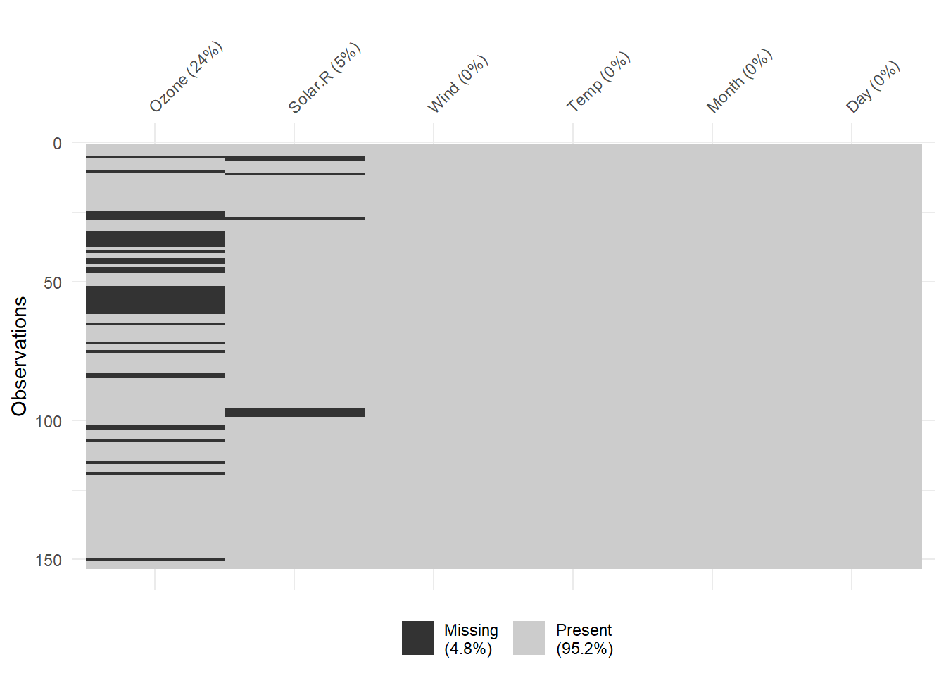
Heatmaps: Highlight where missingness occurs in a dataset.
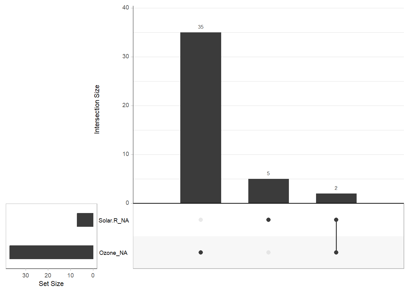
Correlation Plots: Show relationships between missingness indicators of different variables.
Exploring Univariate and Multivariate Missingness
- Univariate Analysis: Calculate the proportion of missing data for each variable.
# Example: Proportion of missing values
missing_proportions <- colSums(is.na(airquality)) / nrow(airquality)
print(missing_proportions)
#>      Ozone    Solar.R       Wind       Temp      Month        Day
#> 0.24183007 0.04575163 0.00000000 0.00000000 0.00000000 0.00000000- Multivariate Analysis: Examine whether missingness in one variable is related to others. This can be visualized using scatterplots of observed vs. missing values.

Figure 13.2: Missing Data Heatmap

Figure 13.3: Missing Data Barchart
13.3.2 Statistical Tests for Missing Data Mechanisms
13.3.2.1 Diagnosing MCAR: Little’s Test
Little’s test is a hypothesis test to determine if the missing data mechanism is MCAR. It tests whether the means of observed and missing data are significantly different. The null hypothesis is that the data are MCAR.
\[ \chi^2 = \sum_{i=1}^n \frac{(O_i - E_i)^2}{E_i} \]
Where:
\(O_i\)= Observed frequency
\(E_i\)= Expected frequency under MCAR
13.3.2.2 Diagnosing MCAR via Dummy Variables
Creating a binary indicator for missingness allows you to test whether the presence of missing data is related to observed data. For instance:
Create a dummy variable:
1 = Missing
0 = Observed
Conduct a chi-square test or t-test:
Chi-square: Compare proportions of missingness across groups.
T-test: Compare means of (other) observed variables with missingness indicators.
# Example: Chi-square test
airquality$missing_var <- as.factor(ifelse(is.na(airquality$Ozone), 1, 0))
# Across groups of months
table(airquality$missing_var, airquality$Month)
#>
#>      5  6  7  8  9
#>   0 26  9 26 26 29
#>   1  5 21  5  5  1
chisq.test(table(airquality$missing_var, airquality$Month))
#>
#>  Pearson's Chi-squared test
#>
#> data:  table(airquality$missing_var, airquality$Month)
#> X-squared = 44.751, df = 4, p-value = 4.48e-09

# Example: T-test (of other variable)
t.test(Wind ~ missing_var, data = airquality)
#>
#>  Welch Two Sample t-test
#>
#> data:  Wind by missing_var
#> t = -0.60911, df = 63.646, p-value = 0.5446
#> alternative hypothesis: true difference in means between group 0 and group 1 is not equal to 0
#> 95 percent confidence interval:
#>  -1.6893132  0.8999377
#> sample estimates:
#> mean in group 0 mean in group 1
#>        9.862069       10.256757
13.3.3 Assessing MAR and MNAR
13.3.3.1 Sensitivity Analysis
Sensitivity analysis involves simulating different scenarios of missing data and assessing how the results change. For example, imputing missing values under different assumptions can provide insight into whether the data are MAR or MNAR.
13.3.3.2 Proxy Variables and External Data
Using proxy variables or external data sources can help assess whether missingness depends on unobserved variables (MNAR). For example, in surveys, follow-ups with non-respondents can reveal systematic differences.
13.3.3.3 Practical Challenges in Distinguishing MAR from MNAR
Distinguishing between Missing at Random (MAR) and Missing Not at Random (MNAR) is a critical and challenging task in data analysis. Properly identifying the nature of the missing data has significant implications for the choice of imputation strategies, model robustness, and the validity of conclusions. While statistical tests can sometimes aid in this determination, the process often relies heavily on domain knowledge, intuition, and exploratory analysis. Below, we discuss key considerations and examples that highlight these challenges:
Sensitive Topics: Missing data related to sensitive or stigmatized topics, such as income, drug use, or health conditions, are often MNAR. For example, individuals with higher incomes might deliberately choose not to report their earnings due to privacy concerns. Similarly, participants in a health survey may avoid answering questions about smoking if they perceive social disapproval. In such cases, the probability of missingness is directly related to the unobserved value itself, making MNAR likely.
Field-Specific Norms: Understanding norms and typical data collection practices in a specific field can provide insights into missingness patterns. For instance, in marketing surveys, respondents may skip questions about spending habits if they consider the questions intrusive. Prior research or historical data from the same domain can help infer whether missingness is more likely MAR (e.g., random skipping due to survey fatigue) or MNAR (e.g., deliberate omission by higher spenders).
Analyzing Auxiliary Variables: Leveraging auxiliary variables—those correlated with the missing variable—can help infer the missingness mechanism. For example, if missing income data strongly correlates with employment status, this suggests a MAR mechanism, as the missingness depends on observed variables. However, if missingness persists even after accounting for observable predictors, MNAR might be at play.
Experimental Design and Follow-Up: In longitudinal studies, dropout rates can signal MAR or MNAR patterns. For example, if dropouts occur disproportionately among participants reporting lower satisfaction in early surveys, this indicates an MNAR mechanism. Designing follow-up surveys to specifically investigate dropout reasons can clarify missingness patterns.
Sensitivity Analysis: To account for uncertainty in the missingness mechanism, researchers can conduct sensitivity analyses by comparing results under different assumptions (e.g., imputing data using both MAR and MNAR approaches). This process helps to quantify the potential impact of misclassifying the missingness mechanism on study conclusions.
Real-World Examples:
- In customer feedback surveys, higher ratings might be overrepresented due to non-response bias. Customers with negative experiences might be less likely to complete surveys, leading to an MNAR scenario.
- In financial reporting, missing audit data might correlate with companies in financial distress, a classic MNAR case where the missingness depends on unobserved financial health metrics.
Summary
MCAR: No pattern in missingness; use Little’s test or dummy variable analysis.
MAR: Missingness related to observed data; requires modeling assumptions or proxy analysis.
MNAR: Missingness depends on unobserved data; requires external validation or sensitivity analysis.