44.4 Demonstration
###############################################################
# HPC Workflow Demo in R: Scaling Resources and Parallelism
###############################################################


# -- 1. Libraries --
library(parallel)       # base parallel
library(doParallel)     # foreach backend
library(foreach)        # parallel loops
library(future)         # futures
library(future.apply)   # apply with futures
library(ggplot2)        # plotting results

# Optional: install.packages("pryr") for memory usage (optional)
# library(pryr)

###############################################################
# -- 2. Generate or Load Data (Small and Large for Scaling) --
###############################################################

set.seed(42)

n_small <- 1e4    # Small dataset (test)
n_large <- 1e6    # Large dataset (scale-up demo)

generate_data <- function(n) {
    data.frame(
        id = 1:n,
        x = rnorm(n, mean = 50, sd = 10),
        y = rnorm(n, mean = 100, sd = 25)
    )
}

data_small <- generate_data(n_small)
data_large <- generate_data(n_large)

###############################################################
# -- 3. Preprocessing Function --
###############################################################

clean_and_transform <- function(df) {
    df$dist <- sqrt(df$x ^ 2 + df$y ^ 2)
    return(df)
}

data_small_clean <- clean_and_transform(data_small)
data_large_clean <- clean_and_transform(data_large)

###############################################################
# -- 4. Heavy Computation (Simulated Workload) --
###############################################################

heavy_computation <- function(df, reps = 500) {
    replicate(reps, sum(df$dist))
}

###############################################################
# -- 5. Resource Measurement Helper Function --
###############################################################

measure_resources <-
    function(expr, approach_name, data_size, cores) {
        start_time <- Sys.time()

        # baseline_mem <- pryr::mem_used()  # If pryr is available
        result <- eval(expr)
        end_time <- Sys.time()

        time_elapsed <-
            as.numeric(difftime(end_time, start_time, units = "secs"))
        # used_mem <- as.numeric(pryr::mem_used() - baseline_mem) / 1e6  # MB

        # If pryr isn't available, approximate:
        used_mem <- as.numeric(object.size(result)) / 1e6  # MB

        return(
            data.frame(
                Approach = approach_name,
                Data_Size = data_size,
                Cores = cores,
                Time_Sec = time_elapsed,
                Memory_MB = round(used_mem, 2)
            )
        )
    }

###############################################################
# -- 6. Define and Run Parallel Approaches --
###############################################################

# Collect results in a dataframe
results <- data.frame()

### 6.1 Single Core (Baseline)
res_single_small <- measure_resources(
    expr = quote(heavy_computation(data_small_clean)),
    approach_name = "SingleCore",
    data_size = nrow(data_small_clean),
    cores = 1
)

res_single_large <- measure_resources(
    expr = quote(heavy_computation(data_large_clean)),
    approach_name = "SingleCore",
    data_size = nrow(data_large_clean),
    cores = 1
)

results <- rbind(results, res_single_small, res_single_large)

# clusterExport(cl, varlist = c("heavy_computation"))


### 6.2 Base Parallel (Cross-Platform): parLapply (Cluster Based)
cores_to_test <- c(2, 4)

for (cores in cores_to_test) {
    cl <- makeCluster(cores)

    # Export both the heavy function and the datasets
    clusterExport(cl,
                  varlist = c(
                      "heavy_computation",
                      "data_small_clean",
                      "data_large_clean"
                  ))

    res_par_small <- measure_resources(
        expr = quote({
            parLapply(
                cl = cl,
                X = 1:cores,
                fun = function(i)
                    heavy_computation(data_small_clean)
            )
        }),
        approach_name = "parLapply",
        data_size = nrow(data_small_clean),
        cores = cores
    )

    res_par_large <- measure_resources(
        expr = quote({
            parLapply(
                cl = cl,
                X = 1:cores,
                fun = function(i)
                    heavy_computation(data_large_clean)
            )
        }),
        approach_name = "parLapply",
        data_size = nrow(data_large_clean),
        cores = cores
    )

    stopCluster(cl)

    results <- rbind(results, res_par_small, res_par_large)
}


### 6.3 foreach + doParallel
for (cores in cores_to_test) {
    cl <- makeCluster(cores)
    registerDoParallel(cl)

    clusterExport(cl,
                  varlist = c(
                      "heavy_computation",
                      "data_small_clean",
                      "data_large_clean"
                  ))
    registerDoParallel(cl)

    # Small dataset
    res_foreach_small <- measure_resources(
        expr = quote({
            foreach(i = 1:cores, .combine = c) %dopar% {
                heavy_computation(data_small_clean)
            }
        }),
        approach_name = "foreach_doParallel",
        data_size = nrow(data_small_clean),
        cores = cores
    )

    # Large dataset
    res_foreach_large <- measure_resources(
        expr = quote({
            foreach(i = 1:cores, .combine = c) %dopar% {
                heavy_computation(data_large_clean)
            }
        }),
        approach_name = "foreach_doParallel",
        data_size = nrow(data_large_clean),
        cores = cores
    )

    stopCluster(cl)

    results <- rbind(results, res_foreach_small, res_foreach_large)
}

### 6.4 future + future.apply
for (cores in cores_to_test) {
    plan(multicore, workers = cores)  # multicore only works on Unix; use multisession on Windows

    # Small dataset
    res_future_small <- measure_resources(
        expr = quote({
            future_lapply(1:cores, function(i)
                heavy_computation(data_small_clean))
        }),
        approach_name = "future_lapply",
        data_size = nrow(data_small_clean),
        cores = cores
    )

    # Large dataset
    res_future_large <- measure_resources(
        expr = quote({
            future_lapply(1:cores, function(i)
                heavy_computation(data_large_clean))
        }),
        approach_name = "future_lapply",
        data_size = nrow(data_large_clean),
        cores = cores
    )

    results <- rbind(results, res_future_small, res_future_large)
}

# Reset plan to sequential
plan(sequential)

###############################################################
# -- 7. Summarize and Plot Results --
###############################################################

# Print table
print(results)
#>              Approach Data_Size Cores   Time_Sec Memory_MB
#> 1          SingleCore     10000     1 0.01586890      0.00
#> 2          SingleCore   1000000     1 1.34883380      0.00
#> 3           parLapply     10000     2 0.01907897      0.01
#> 4           parLapply   1000000     2 1.33863306      0.01
#> 5           parLapply     10000     4 0.01780701      0.02
#> 6           parLapply   1000000     4 1.32461405      0.02
#> 7  foreach_doParallel     10000     2 0.05314898      0.01
#> 8  foreach_doParallel   1000000     2 1.33675098      0.01
#> 9  foreach_doParallel     10000     4 0.06010795      0.02
#> 10 foreach_doParallel   1000000     4 1.34139991      0.02
#> 11      future_lapply     10000     2 0.09521294      0.01
#> 12      future_lapply   1000000     2 2.73076987      0.01
#> 13      future_lapply     10000     4 0.10914207      0.02
#> 14      future_lapply   1000000     4 5.50541496      0.02

# Save to CSV
# write.csv(results, "HPC_parallel_results.csv", row.names = FALSE)

# Plot Time vs. Data Size / Cores
ggplot(results, aes(x = as.factor(Cores), y = Time_Sec, fill = Approach)) +
    geom_bar(stat = "identity", position = "dodge") +
    facet_wrap( ~ Data_Size, scales = "free", labeller = label_both) +
    labs(title = "Runtime by Cores, Approach, and Data Size",
         x = "Number of Cores",
         y = "Time (Seconds)") +
    theme_minimal()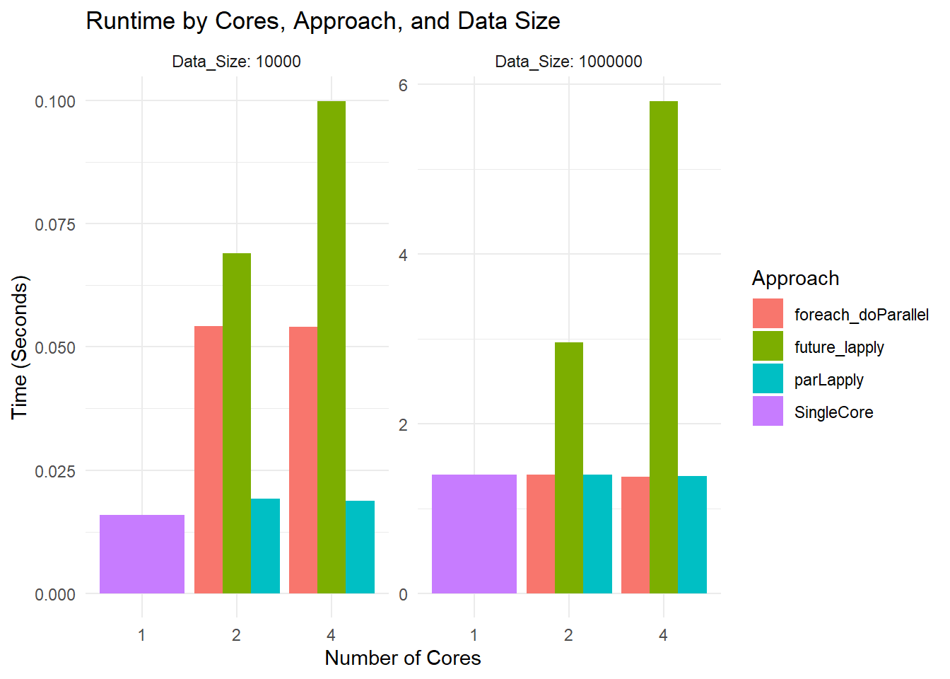
# Plot Memory Usage
ggplot(results, aes(x = as.factor(Cores), y = Memory_MB, fill = Approach)) +
    geom_bar(stat = "identity", position = "dodge") +
    facet_wrap(~ Data_Size, scales = "free", labeller = label_both) +
    labs(title = "Memory Usage by Cores, Approach, and Data Size",
         x = "Number of Cores",
         y = "Memory (MB)") +
    theme_minimal()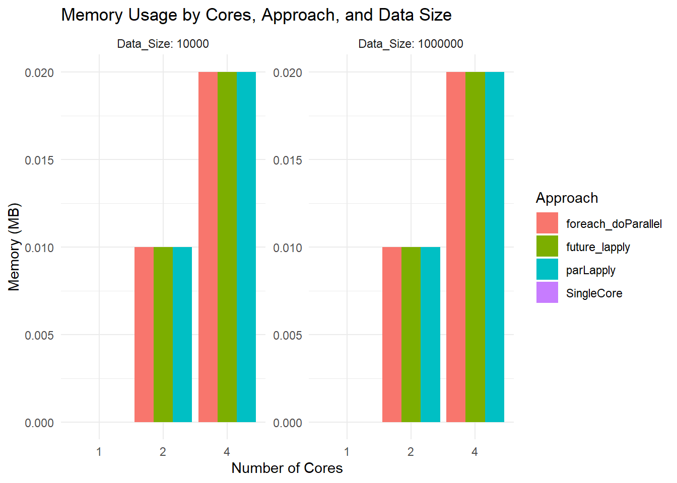
Runtime Plot
Small Dataset: All methods are so fast that you are mostly seeing overhead differences. The differences in bar heights reflect how each parallel framework handles overhead.
Large Dataset: You see more separation. For instance,
parLapplywith 2 cores might be slower than 1 core due to overhead. At 4 cores, it might improve or not, depending on how the overhead and actual workload balance out.
Memory Usage Plot
- All bars hover around 0.02 MB or so because you are measuring the size of the returned result, not the in-memory size of the large dataset. The function
object.size(result)is not capturing total RAM usage by the entire parallel job.
- All bars hover around 0.02 MB or so because you are measuring the size of the returned result, not the in-memory size of the large dataset. The function