37.3 Survivorship Bias
Survivorship bias refers to the logical error of concentrating on the entities that have made it past some selection process and overlooking those that didn’t, typically because of a lack of visibility. This can skew results and lead to overly optimistic conclusions.
Example: If you were to analyze the success of companies based only on the ones that are still in business today, you’d miss out on the insights from all those that failed. This would give you a distorted view of what makes a successful company, as you wouldn’t account for all those that had those same attributes but didn’t succeed.
Relation to Other Biases:
Sample Selection Bias: Survivorship bias is a specific form of sample selection bias. While survivorship bias focuses on entities that “survive”, sample selection bias broadly deals with any non-random sample.
Confirmation Bias: Survivorship bias can reinforce confirmation bias. By only looking at the “winners”, we might confirm our existing beliefs about what leads to success, ignoring evidence to the contrary from those that didn’t survive.
set.seed(42)

# Generating data for 100 companies
n <- 100

# Randomly generate earnings; assume true average earnings is 50
earnings <- rnorm(n, mean = 50, sd = 10)

# Threshold for bankruptcy
threshold <- 40

# Only companies with earnings above the threshold "survive"
survivor_earnings <- earnings[earnings > threshold]

# Average earnings for all companies vs. survivors
true_avg <- mean(earnings)
survivor_avg <- mean(survivor_earnings)

true_avg
#> [1] 50.32515
survivor_avg
#> [1] 53.3898
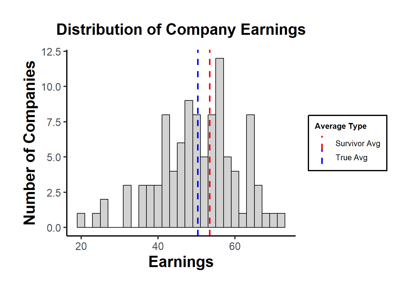
Using a histogram to visualize the distribution of earnings, highlighting the “survivors”.
library(ggplot2)

df <- data.frame(earnings)

p <- ggplot(df, aes(x = earnings)) +
  geom_histogram(
    binwidth = 2,
    fill = "grey",
    color = "black",
    alpha = 0.7
  ) +
  geom_vline(aes(xintercept = true_avg, color = "True Avg"),
             linetype = "dashed",
             size = 1) +
  geom_vline(
    aes(xintercept = survivor_avg, color = "Survivor Avg"),
    linetype = "dashed",
    size = 1
  ) +
  scale_color_manual(values = c("True Avg" = "blue", "Survivor Avg" = "red"),
                     name = "Average Type") +
  labs(title = "Distribution of Company Earnings",
       x = "Earnings",
       y = "Number of Companies") +
  causalverse::ama_theme()

print(p)
In the plot, the “True Avg” might be lower than the “Survivor Avg”, indicating that by only looking at the survivors, we overestimate the average earnings.
Remedies:
Awareness: Recognizing the potential for survivorship bias is the first step.
Inclusive Data Collection: Wherever possible, try to include data from entities that didn’t “survive” in your sample.
Statistical Techniques: In cases where the missing data is inherent, methods like Heckman’s two-step procedure can be used to correct for sample selection bias.
External Data Sources: Sometimes, complementary datasets can provide insights into the missing “non-survivors”.
Sensitivity Analysis: Test how sensitive your results are to assumptions about the non-survivors.