Appendix: Reproducible Snippets
# jtools: baseline summary again for traceability data (movies)<- lm (metascore ~ budget + us_gross + year, data = movies)summ (fit)
Observations
831 (10 missing obs. deleted)
Dependent variable
metascore
Type
OLS linear regression
F(3,827)
26.23
R²
0.09
Adj. R²
0.08
Est.
S.E.
t val.
p
(Intercept)
52.06
139.67
0.37
0.71
budget
-0.00
0.00
-5.89
0.00
us_gross
0.00
0.00
7.61
0.00
year
0.01
0.07
0.08
0.94
summ (scale = TRUE ,vifs = TRUE ,part.corr = TRUE ,confint = TRUE ,pvals = FALSE # notice that scale here is TRUE
Observations
831 (10 missing obs. deleted)
Dependent variable
metascore
Type
OLS linear regression
F(3,827)
26.23
R²
0.09
Adj. R²
0.08
Est.
2.5%
97.5%
t val.
VIF
partial.r
part.r
(Intercept)
63.01
61.91
64.11
112.23
NA
NA
NA
budget
-3.78
-5.05
-2.52
-5.89
1.31
-0.20
-0.20
us_gross
5.28
3.92
6.64
7.61
1.52
0.26
0.25
year
0.05
-1.18
1.28
0.08
1.24
0.00
0.00
# obtain cluster-robust SE data ("PetersenCL" , package = "sandwich" )<- lm (y ~ x, data = PetersenCL)summ (fit2, robust = "HC3" , cluster = "firm" )
Observations
5000
Dependent variable
y
Type
OLS linear regression
F(1,4998)
1310.74
R²
0.21
Adj. R²
0.21
Est.
S.E.
t val.
p
(Intercept)
0.03
0.07
0.44
0.66
x
1.03
0.05
20.36
0.00
# Model to Equation via equatiomatic (if available) # install.packages("equatiomatic") # not available for R 4.2 <- lm (metascore ~ budget + us_gross + year, data = movies)# show the theoretical model :: extract_eq (fit)# display the actual coefficients :: extract_eq (fit, use_coefs = TRUE )# Model Comparison via jtools <- lm (metascore ~ log (budget), data = movies)<- lm (metascore ~ log (budget) + log (us_gross), data = movies)<- lm (metascore ~ log (budget) + log (us_gross) + runtime, data = movies)<- c ("Budget" = "log(budget)" , "US Gross" = "log(us_gross)" ,"Runtime (Hours)" = "runtime" , "Constant" = "(Intercept)" )export_summs (fit, fit_b, fit_c, robust = "HC3" , coefs = coef_names)
-2.43 *** -5.16 *** -6.70 ***
(0.44) (0.62) (0.67)
3.96 *** 3.85 ***
(0.51) (0.48)
14.29 ***
(1.63)
105.29 *** 81.84 *** 83.35 ***
(7.65) (8.66) (8.82)
831 831 831
0.03 0.09 0.17
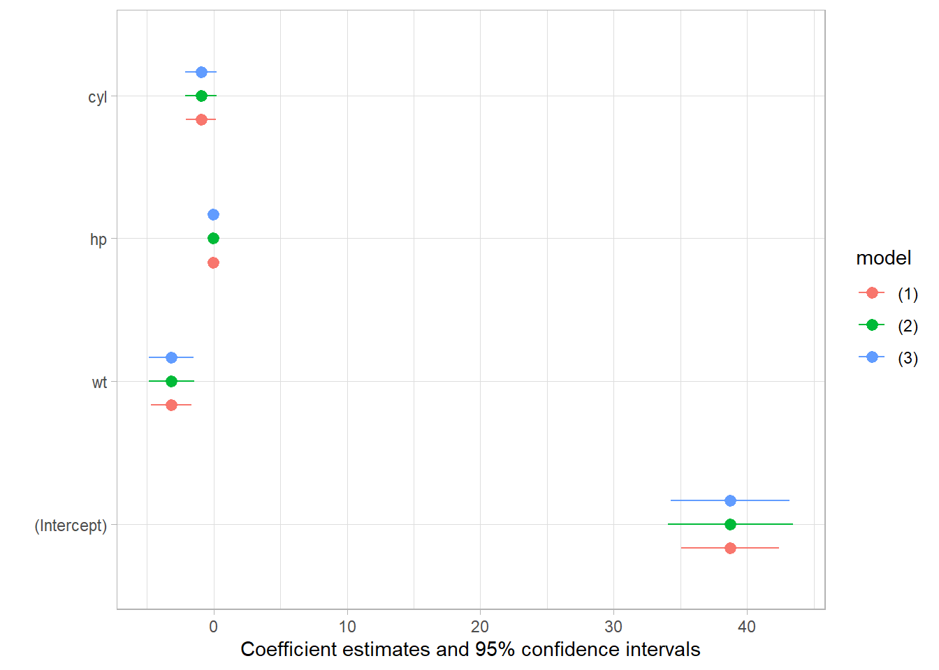
# modelsummary quick demo library (modelsummary)<- lm (mpg ~ wt + hp + cyl, mtcars)msummary (lm_mod, vcov = c ("iid" ,"robust" ,"HC4" ))
(1)
(2)
(3)
(Intercept)
38.752
38.752
38.752
(1.787)
(2.286)
(2.177)
wt
-3.167
-3.167
-3.167
(0.741)
(0.833)
(0.819)
hp
-0.018
-0.018
-0.018
(0.012)
(0.010)
(0.013)
cyl
-0.942
-0.942
-0.942
(0.551)
(0.573)
(0.572)
Num.Obs.
32
32
32
R2
0.843
0.843
0.843
R2 Adj.
0.826
0.826
0.826
AIC
155.5
155.5
155.5
BIC
162.8
162.8
162.8
Log.Lik.
-72.738
-72.738
-72.738
F
50.171
31.065
32.623
RMSE
2.35
2.35
2.35
Std.Errors
IID
HC3
HC4
modelplot (lm_mod, vcov = c ("iid" ,"robust" ,"HC4" ))
# stargazer examples (as in text) library ("stargazer" )stargazer (attitude).1 <- lm (rating ~ complaints + privileges + learning + raises + critical,data = attitude).2 <- lm (rating ~ complaints + privileges + learning, data = attitude)$ high.rating <- (attitude$ rating > 70 )<- glm (~ learning + critical + advance,data = attitude,family = binomial (link = "probit" )stargazer (linear.1 ,.2 ,title = "Results" ,align = TRUE )# LaTeX-ready stargazer (as in text) stargazer (.1 ,.2 ,title = "Regression Results" ,align = TRUE ,dep.var.labels = c ("Overall Rating" , "High Rating" ),covariate.labels = c ("Handling of Complaints" ,"No Special Privileges" ,"Opportunity to Learn" ,"Performance-Based Raises" ,"Too Critical" ,"Advancement" omit.stat = c ("LL" , "ser" , "f" ),no.space = TRUE # ASCII text output (as in text) stargazer (.1 ,.2 ,type = "text" ,title = "Regression Results" ,dep.var.labels = c ("Overall Rating" , "High Rating" ),covariate.labels = c ("Handling of Complaints" ,"No Special Privileges" ,"Opportunity to Learn" ,"Performance-Based Raises" ,"Too Critical" ,"Advancement" omit.stat = c ("LL" , "ser" , "f" ),ci = TRUE ,ci.level = 0.90 ,single.row = TRUE #> #> Regression Results #> ======================================================================== #> Dependent variable: #> ----------------------------------------------- #> Overall Rating #> (1) (2) #> ------------------------------------------------------------------------ #> Handling of Complaints 0.692*** (0.447, 0.937) 0.682*** (0.470, 0.894) #> No Special Privileges -0.104 (-0.325, 0.118) -0.103 (-0.316, 0.109) #> Opportunity to Learn 0.249 (-0.013, 0.512) 0.238* (0.009, 0.467) #> Performance-Based Raises -0.033 (-0.366, 0.299) #> Too Critical 0.015 (-0.227, 0.258) #> Advancement 11.011 (-8.240, 30.262) 11.258 (-0.779, 23.296) #> ------------------------------------------------------------------------ #> Observations 30 30 #> R2 0.715 0.715 #> Adjusted R2 0.656 0.682 #> ======================================================================== #> Note: *p<0.1; **p<0.05; ***p<0.01 # Correlation table <- cor (attitude[, c ("rating" , "complaints" , "privileges" )])stargazer (correlation.matrix, title = "Correlation Matrix" )Pro Tip: Save figures reproducibly for journals:
ggsave (filename = file.path ('output' ,'coef_plot.png' ),plot = last_plot (),width = 6.5 , height = 4.5 , dpi = 300 )