30.8 Staggered Difference-in-Differences

In settings where treatment is introduced at different times across units—known as staggered treatment adoption—researchers often use staggered DiD designs (sometimes called event-study DiD or dynamic DiD). However, standard TWFE regression methods can lead to biased estimates in these contexts due to treatment effect heterogeneity and variation in treatment timing.

For applied guidance, see (Wing et al. 2024) and recommendations in (Baker, Larcker, and Wang 2022).

Best Practices and Recommendations

When is TWFE Appropriate?

Single Treatment Period
TWFE DiD regressions are suitable when there is only one treatment period (i.e., no variation in treatment timing).
Homogeneous Treatment Effects
If there is a strong theoretical rationale to assume that treatment effects are homogeneous across cohorts and over time, TWFE may still be appropriate.

Diagnosing and Addressing Bias in TWFE with Staggered Adoption

Plot Treatment Timing
Examine the distribution of treatment timing across units. Heterogeneous timing suggests high risk of bias in standard TWFE regressions.
Decomposition Methods
Use decomposition approaches, such as (Goodman-Bacon 2021), to understand the weights TWFE places on treatment effects across cohorts and time.
- If decomposition is infeasible (e.g., unbalanced panels), the share of never-treated units can indicate potential bias severity.
Discuss Treatment Effect Heterogeneity
Researchers should explicitly discuss the likelihood and nature of treatment effect heterogeneity.

Event-Study Specifications with TWFE

Avoid Arbitrary Binning
Do not collapse or bin time periods unless you can justify homogeneity in effects.
Full Relative-Time Indicators
Include fully flexible relative time indicators, and justify the reference period (usually $l = -1$ or the period just prior to treatment).
Multicollinearity and Bias
Be cautious about multicollinearity when including leads and lags, which can bias estimates and lead to false detection of pre-trends.

Alternative Estimators to Address Bias

Stacked Regressions
(Callaway and Sant’Anna 2021): Group-Time Average Treatment Effects
(L. Sun and Abraham 2021): Event-Study DiD with clean controls

Alternative methods provide unbiased estimates of ATT even with staggered adoption and heterogeneous effects.

Example of a Basic TWFE Event-Study Specification

Adapted from (Stevenson and Wolfers 2006):

$\begin{aligned} Y_{it} &= \sum_k \beta_k \cdot Treatment_{it}^k + \eta_i + \lambda_t + Controls_{it} + \epsilon_{it} \end{aligned}$

$Treatment_{it}^k$ : Dummy variables equal to 1 if unit $i$ is treated $k$ years before period $t$ .
$\eta_i$ : Unit fixed effects controlling for time-invariant heterogeneity.
$\lambda_t$ : Time fixed effects controlling for common shocks.
Standard Errors (SE): Typically clustered at the group level (e.g., state or cohort).

Common practice: Drop the period immediately before treatment to avoid perfect multicollinearity.

30.8.1 Cohort Average Treatment Effects (L. Sun and Abraham 2021)

L. Sun and Abraham (2021) propose a solution to the TWFE problem in staggered adoption settings by introducing an interaction-weighted estimator for dynamic treatment effects. This estimator is based on the concept of Cohort Average Treatment Effects on the Treated (CATT), which accounts for variation in treatment timing and dynamic treatment responses.

Traditional TWFE estimators implicitly assume homogeneous treatment effects and often rely on treated units serving as controls for later-treated units. When treatment effects vary over time or across groups, this leads to contaminated comparisons, especially in event-study specifications.

L. Sun and Abraham (2021) address this issue by:

Estimating cohort-specific treatment effects relative to time since treatment.
Using never-treated units as controls, or in their absence, the last-treated cohort.

30.8.1.1 Defining the Parameter of Interest: CATT

Let $E_i = e$ denote the period when unit $i$ first receives treatment. The cohort-specific average treatment effect on the treated (CATT) is defined as: $CATT_{e, l} = \mathbb{E}[Y_{i, e + l} - Y_{i, e + l}^\infty \mid E_i = e]$ Where:

$l$ is the relative period (e.g., $l = -1$ is one year before treatment, $l = 0$ is the treatment year).
$Y_{i, e + l}^\infty$ is the potential outcome without treatment.
$Y_{i, e + l}$ is the observed outcome.

This formulation allows one to trace out the dynamic effect of treatment for each cohort, relative to their treatment start time.

L. Sun and Abraham (2021) extend the interaction-weighted idea to panel settings, originally introduced by Gibbons, Suárez Serrato, and Urbancic (2018) in a cross-sectional context.

They propose regressing the outcome on:

Relative time indicators constructed by interacting treatment cohort ( $E_i$ ) with time ( $t$ ).
Unit and time fixed effects.

This method explicitly estimates $CATT_{e, l}$ terms, avoiding the contaminating influence of already-treated units that TWFE models often suffer from.

Relative Period Bin Indicator

$D_{it}^l = \mathbb{1}(t - E_i = l)$

$E_i$ : The time period when unit $i$ first receives treatment.
$l$ : The relative time period—how many periods have passed since treatment began.

Static Specification

$Y_{it} = \alpha_i + \lambda_t + \mu_g \sum_{l \ge 0} D_{it}^l + \epsilon_{it}$

$\alpha_i$ : Unit fixed effects.
$\lambda_t$ : Time fixed effects.
$\mu_g$ : Effect for group $g$ .
Excludes periods prior to treatment.

Dynamic Specification

$Y_{it} = \alpha_i + \lambda_t + \sum_{\substack{l = -K \\ l \neq -1}}^{L} \mu_l D_{it}^l + \epsilon_{it}$

Includes leads and lags of treatment indicators $D_{it}^l$ .
Excludes one period (typically $l = -1$ ) to avoid perfect collinearity.
Tests for pre-treatment parallel trends rely on the leads ( $l < 0$ ).

30.8.1.2 Identifying Assumptions

Parallel Trends

For identification, it is assumed that untreated potential outcomes follow parallel trends across cohorts in the absence of treatment: $\mathbb{E}[Y_{it}^\infty - Y_{i, t-1}^\infty \mid E_i = e] = \text{constant across } e$ This allows us to use never-treated or not-yet-treated units as valid counterfactuals.

No Anticipatory Effects

Treatment should not influence outcomes before it is implemented. That is: $CATT_{e, l} = 0 \quad \text{for all } l < 0$ This ensures that any pre-trends are not driven by behavioral changes in anticipation of treatment.

Treatment Effect Homogeneity (Optional)

The treatment effect is consistent across cohorts for each relative period. Each adoption cohort should have the same path of treatment effects. In other words, the trajectory of each treatment cohort is similar.

Although L. Sun and Abraham (2021) allow treatment effect heterogeneity, some settings may assume homogeneous effects within cohorts and periods:

Each cohort has the same pattern of response over time.
This is relaxed in their design but assumed in simpler TWFE settings.

30.8.1.3 Comparison to Other Designs

Different DiD designs make distinct assumptions about how treatment effects vary:

Study	Vary Over Time	Vary Across Cohorts	Notes
L. Sun and Abraham (2021)	✓	✓	Allows full heterogeneity
Callaway and Sant’Anna (2021)	✓	✓	Estimates group × time ATTs
Borusyak, Jaravel, and Spiess (2024)	✓	✗	Homogeneous across cohorts Heterogeneity over time
Athey and Imbens (2022)	✗	✓	Heterogeneity only across adoption cohorts
Clement De Chaisemartin and D’haultfœuille (2023)	✓	✓	Complete heterogeneity
Goodman-Bacon (2021)	✓ or ✗	✗ or ✓	Restricts one dimension Heterogeneity either “vary across units but not over time” or “vary over time but not across units”.

30.8.1.4 Sources of Treatment Effect Heterogeneity

Several forces can generate heterogeneous treatment effects:

Calendar Time Effects: Macro events (e.g., recessions, policy changes) affect cohorts differently.
Selection into Timing: Units self-select into early/late treatment based on anticipated effects.
Composition Differences: Adoption cohorts may differ in observed or unobserved ways.

Such heterogeneity can bias TWFE estimates, which often average effects across incomparable groups.

30.8.1.5 Technical Issues

When using an event-study TWFE regression to estimate dynamic treatment effects in staggered adoption settings, one must exclude certain relative time indicators to avoid perfect multicollinearity. This arises because relative period indicators are linearly dependent due to the presence of unit and time fixed effects.

Specifically, the following two terms must be addressed:

The period immediately before treatment ( $l = -1$ ): This period is typically omitted and serves as the baseline for comparison. This normalization has been standard practice in event study regressions prior to L. Sun and Abraham (2021) .
A distant post-treatment period (e.g., $l = +5$ or $l = +10$ ): L. Sun and Abraham (2021) clarified that in addition to the baseline period, at least one other relative time indicator—typically from the far tail of the post-treatment distribution—must be dropped, binned, or trimmed to avoid multicollinearity among the relative time dummies. This issue emerges because fixed effects absorb much of the within-unit and within-time variation, reducing the effective rank of the design matrix.

Dropping certain relative periods (especially pre-treatment periods) introduces an implicit normalization: the estimates for included periods are now interpreted relative to the omitted periods. If treatment effects are present in these omitted periods—say, due to anticipation or early effects—this will contaminate the estimates of included relative periods.

To avoid this contamination, researchers often assume that all pre-treatment periods have zero treatment effect, i.e.,

$CATT_{e, l} = 0 \quad \text{for all } l < 0$

This assumption ensures that excluded pre-treatment periods form a valid counterfactual, and estimates for $l \geq 0$ are not biased due to normalization.

L. Sun and Abraham (2021) resolve the issues of weighting and aggregation by using a clean weighting scheme that avoids contamination from excluded periods. Their method produces a weighted average of cohort- and time-specific treatment effects ( $CATT_{e, l}$ ), where the weights are:

Non-negative
Sum to one
Interpretable as the fraction of treated units who are observed $l$ periods after treatment, normalized over the number of available periods $g$

This interaction-weighted estimator ensures that the estimated average treatment effect reflects a convex combination of dynamic treatment effects from different cohorts and times.

In this way, their aggregation logic closely mirrors that of Callaway and Sant’Anna (2021), who also construct average treatment effects from group-time ATTs using interpretable weights that align with the sampling structure.

library(fixest)
data("base_stagg")

# Estimate Sun & Abraham interaction-weighted model
res_sa20 <- feols(
  y ~ x1 + sunab(year_treated, year) | id + year,
  data = base_stagg
)

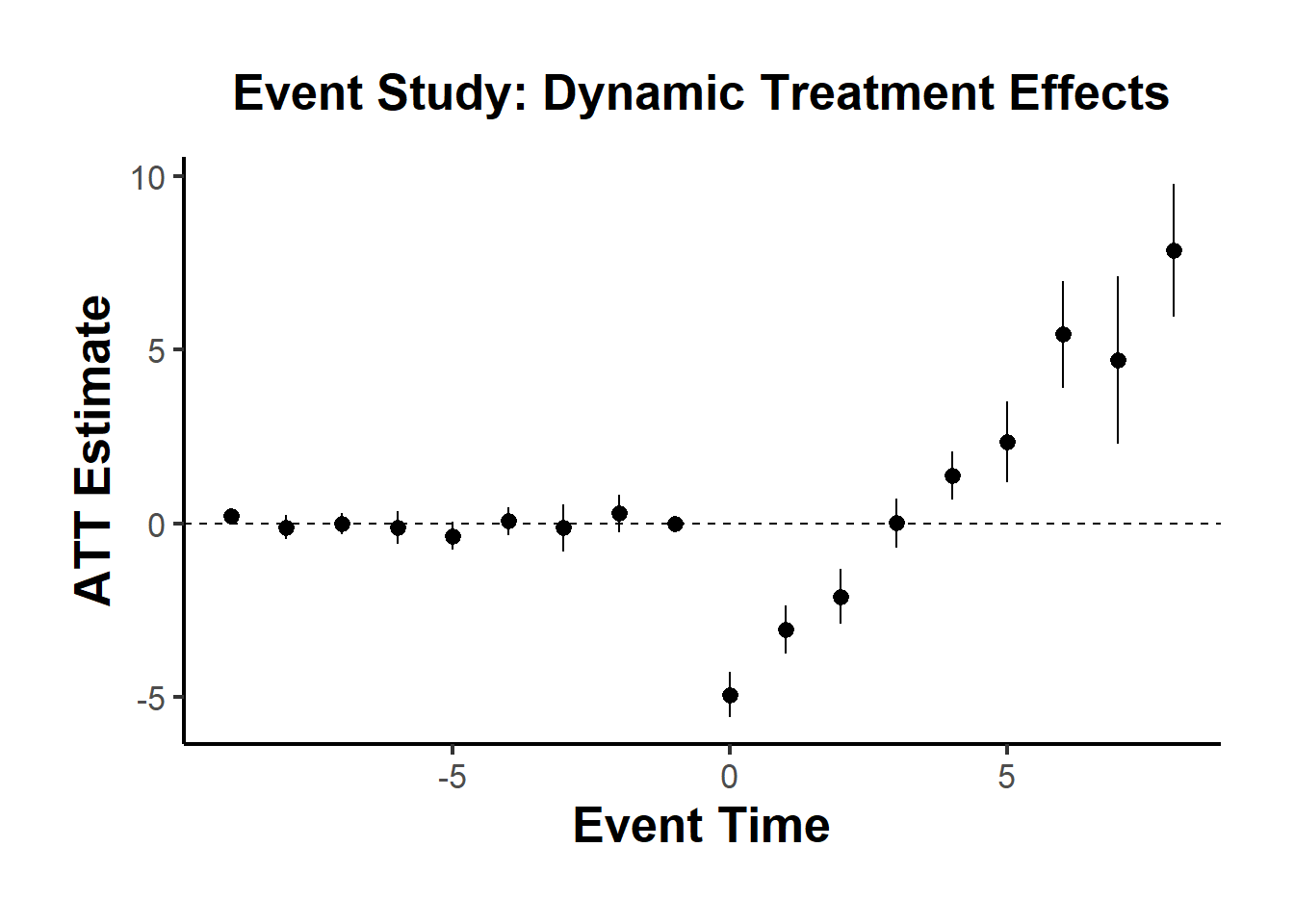
Use iplot() to visualize the estimated dynamic treatment effects across relative time:

iplot(res_sa20)

You can summarize the results using different aggregation options:

# Overall average ATT
summary(res_sa20, agg = "att")
#> OLS estimation, Dep. Var.: y
#> Observations: 950
#> Fixed-effects: id: 95,  year: 10
#> Standard-errors: Clustered (id) 
#>      Estimate Std. Error  t value  Pr(>|t|)    
#> x1   0.994678   0.018378 54.12293 < 2.2e-16 ***
#> ATT -1.133749   0.205070 -5.52858 2.882e-07 ***
#> ---
#> Signif. codes:  0 '***' 0.001 '**' 0.01 '*' 0.05 '.' 0.1 ' ' 1
#> RMSE: 0.921817     Adj. R2: 0.887984
#>                  Within R2: 0.876406

# Aggregation across post-treatment periods (excluding leads)
summary(res_sa20, agg = c("att" = "year::[^-]"))
#> OLS estimation, Dep. Var.: y
#> Observations: 950
#> Fixed-effects: id: 95,  year: 10
#> Standard-errors: Clustered (id) 
#>                      Estimate Std. Error   t value   Pr(>|t|)    
#> x1                   0.994678   0.018378 54.122928  < 2.2e-16 ***
#> year::-9:cohort::10  0.351766   0.359073  0.979649 3.2977e-01    
#> year::-8:cohort::9   0.033914   0.471437  0.071937 9.4281e-01    
#> year::-8:cohort::10 -0.191932   0.352896 -0.543876 5.8781e-01    
#> year::-7:cohort::8  -0.589387   0.736910 -0.799809 4.2584e-01    
#> year::-7:cohort::9   0.872995   0.493427  1.769249 8.0096e-02 .  
#> year::-7:cohort::10  0.019512   0.603411  0.032336 9.7427e-01    
#> year::-6:cohort::7  -0.042147   0.865736 -0.048683 9.6127e-01    
#> year::-6:cohort::8  -0.657571   0.573257 -1.147078 2.5426e-01    
#> year::-6:cohort::9   0.877743   0.533331  1.645775 1.0315e-01    
#> year::-6:cohort::10 -0.403635   0.347412 -1.161832 2.4825e-01    
#> year::-5:cohort::6  -0.658034   0.913407 -0.720418 4.7306e-01    
#> year::-5:cohort::7  -0.316974   0.697939 -0.454158 6.5076e-01    
#> year::-5:cohort::8  -0.238213   0.469744 -0.507113 6.1326e-01    
#> year::-5:cohort::9   0.301477   0.604201  0.498968 6.1897e-01    
#> year::-5:cohort::10 -0.564801   0.463214 -1.219308 2.2578e-01    
#> year::-4:cohort::5  -0.983453   0.634492 -1.549984 1.2451e-01    
#> year::-4:cohort::6   0.360407   0.858316  0.419900 6.7552e-01    
#> year::-4:cohort::7  -0.430610   0.661356 -0.651102 5.1657e-01    
#> year::-4:cohort::8  -0.895195   0.374901 -2.387816 1.8949e-02 *  
#> year::-4:cohort::9  -0.392478   0.439547 -0.892914 3.7418e-01    
#> year::-4:cohort::10  0.519001   0.597880  0.868069 3.8757e-01    
#> year::-3:cohort::4   0.591288   0.680169  0.869324 3.8688e-01    
#> year::-3:cohort::5  -1.000650   0.971741 -1.029749 3.0577e-01    
#> year::-3:cohort::6   0.072188   0.652641  0.110609 9.1216e-01    
#> year::-3:cohort::7  -0.836820   0.804275 -1.040465 3.0079e-01    
#> year::-3:cohort::8  -0.783148   0.701312 -1.116691 2.6697e-01    
#> year::-3:cohort::9   0.811285   0.564470  1.437251 1.5397e-01    
#> year::-3:cohort::10  0.527203   0.320051  1.647250 1.0285e-01    
#> year::-2:cohort::3   0.036941   0.673771  0.054828 9.5639e-01    
#> year::-2:cohort::4   0.832250   0.859544  0.968246 3.3541e-01    
#> year::-2:cohort::5  -1.574086   0.525563 -2.995051 3.5076e-03 ** 
#> year::-2:cohort::6   0.311758   0.832095  0.374666 7.0875e-01    
#> year::-2:cohort::7  -0.558631   0.871993 -0.640638 5.2332e-01    
#> year::-2:cohort::8   0.429591   0.305270  1.407250 1.6265e-01    
#> year::-2:cohort::9   1.201899   0.819186  1.467188 1.4566e-01    
#> year::-2:cohort::10 -0.002429   0.682087 -0.003562 9.9717e-01    
#> att                 -1.133749   0.205070 -5.528584 2.8820e-07 ***
#> ---
#> Signif. codes:  0 '***' 0.001 '**' 0.01 '*' 0.05 '.' 0.1 ' ' 1
#> RMSE: 0.921817     Adj. R2: 0.887984
#>                  Within R2: 0.876406

# Aggregate post-treatment effects from l = 0 to 8
summary(res_sa20, agg = c("att" = "year::[012345678]")) |> 
  etable(digits = 2)
#>                         summary(res_..
#> Dependent Var.:                      y
#>                                       
#> x1                      0.99*** (0.02)
#> year = -9 x cohort = 10    0.35 (0.36)
#> year = -8 x cohort = 9     0.03 (0.47)
#> year = -8 x cohort = 10   -0.19 (0.35)
#> year = -7 x cohort = 8    -0.59 (0.74)
#> year = -7 x cohort = 9    0.87. (0.49)
#> year = -7 x cohort = 10    0.02 (0.60)
#> year = -6 x cohort = 7    -0.04 (0.87)
#> year = -6 x cohort = 8    -0.66 (0.57)
#> year = -6 x cohort = 9     0.88 (0.53)
#> year = -6 x cohort = 10   -0.40 (0.35)
#> year = -5 x cohort = 6    -0.66 (0.91)
#> year = -5 x cohort = 7    -0.32 (0.70)
#> year = -5 x cohort = 8    -0.24 (0.47)
#> year = -5 x cohort = 9     0.30 (0.60)
#> year = -5 x cohort = 10   -0.56 (0.46)
#> year = -4 x cohort = 5    -0.98 (0.63)
#> year = -4 x cohort = 6     0.36 (0.86)
#> year = -4 x cohort = 7    -0.43 (0.66)
#> year = -4 x cohort = 8   -0.90* (0.37)
#> year = -4 x cohort = 9    -0.39 (0.44)
#> year = -4 x cohort = 10    0.52 (0.60)
#> year = -3 x cohort = 4     0.59 (0.68)
#> year = -3 x cohort = 5     -1.0 (0.97)
#> year = -3 x cohort = 6     0.07 (0.65)
#> year = -3 x cohort = 7    -0.84 (0.80)
#> year = -3 x cohort = 8    -0.78 (0.70)
#> year = -3 x cohort = 9     0.81 (0.56)
#> year = -3 x cohort = 10    0.53 (0.32)
#> year = -2 x cohort = 3     0.04 (0.67)
#> year = -2 x cohort = 4     0.83 (0.86)
#> year = -2 x cohort = 5   -1.6** (0.53)
#> year = -2 x cohort = 6     0.31 (0.83)
#> year = -2 x cohort = 7    -0.56 (0.87)
#> year = -2 x cohort = 8     0.43 (0.31)
#> year = -2 x cohort = 9      1.2 (0.82)
#> year = -2 x cohort = 10  -0.002 (0.68)
#> att                     -1.1*** (0.21)
#> Fixed-Effects:          --------------
#> id                                 Yes
#> year                               Yes
#> _______________________ ______________
#> S.E.: Clustered                 by: id
#> Observations                       950
#> R2                             0.90982
#> Within R2                      0.87641
#> ---
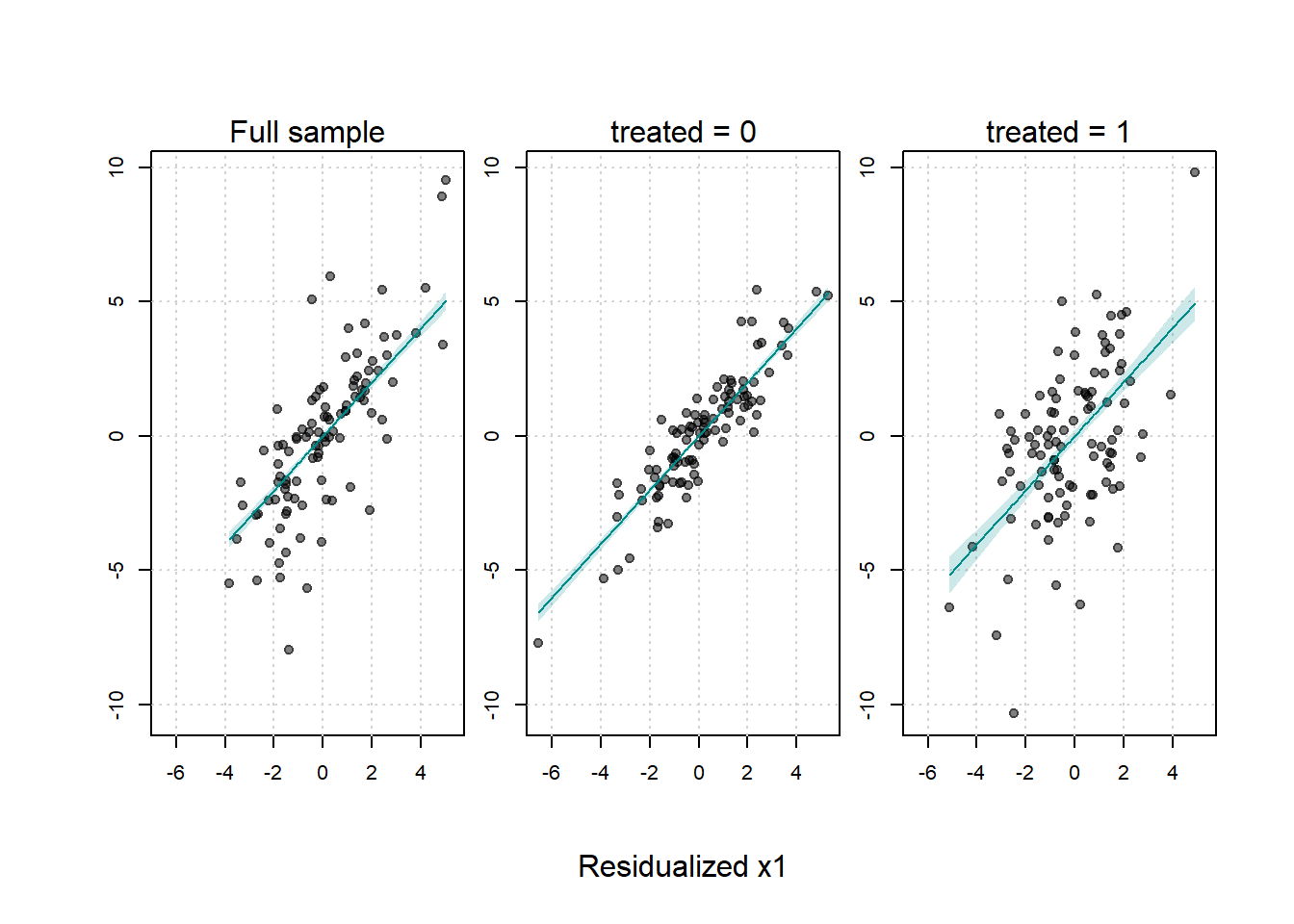
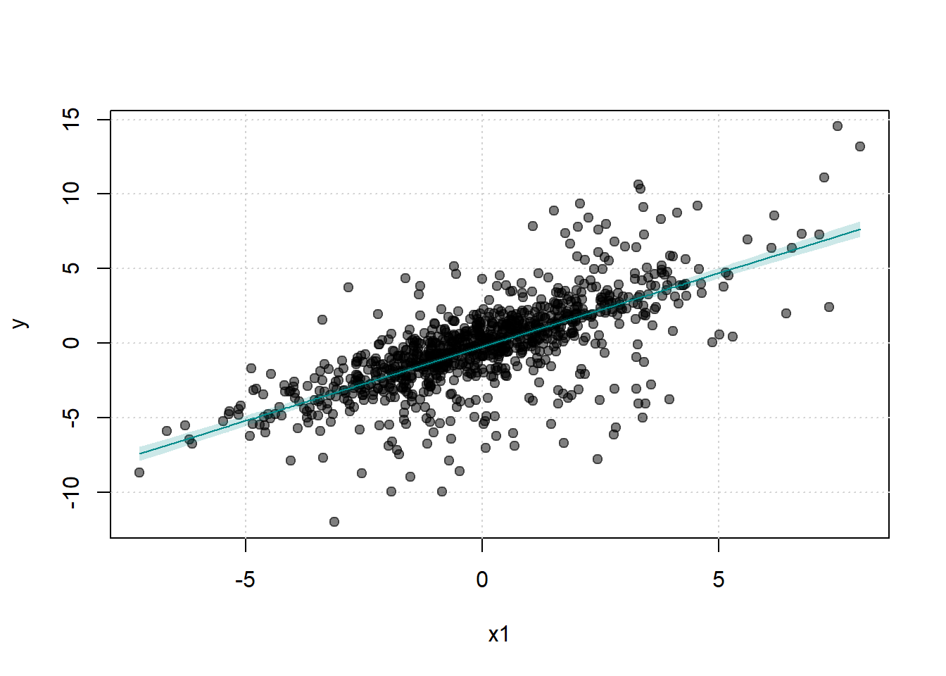
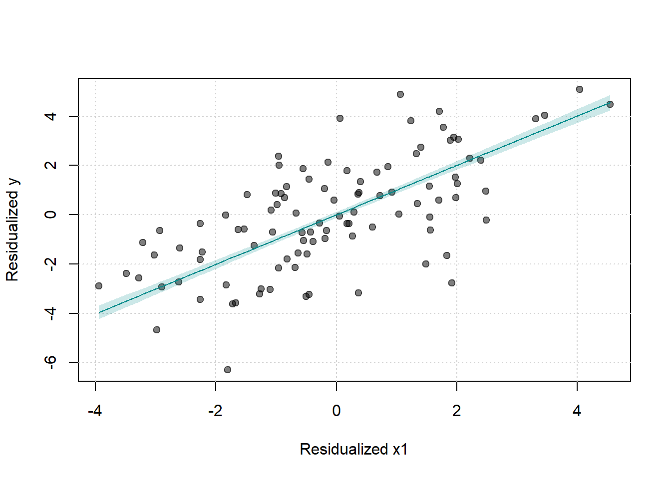
#> Signif. codes: 0 '***' 0.001 '**' 0.01 '*' 0.05 '.' 0.1 ' ' 1

The fwlplot package provides diagnostics for how much variation is explained by fixed effects or covariates:

# Simple FWL plot
fwl_plot(y ~ x1, data = base_stagg)


# With fixed effects
fwl_plot(y ~ x1 | id + year, data = base_stagg, n_sample = 100)


# Splitting by treatment status
fwl_plot(y ~ x1 | id + year, data = base_stagg, n_sample = 100, fsplit = ~ treated)

References

———. 2022. “Design-Based Analysis in Difference-in-Differences Settings with Staggered Adoption.” Journal of Econometrics 226 (1): 62–79.

Baker, Andrew C, David F Larcker, and Charles CY Wang. 2022. “How Much Should We Trust Staggered Difference-in-Differences Estimates?” Journal of Financial Economics 144 (2): 370–95.

———. 2024. “Revisiting Event-Study Designs: Robust and Efficient Estimation.” Review of Economic Studies 91 (6): 3253–85.

Callaway, Brantly, and Pedro HC Sant’Anna. 2021. “Difference-in-Differences with Multiple Time Periods.” Journal of Econometrics 225 (2): 200–230.

De Chaisemartin, Clement, and Xavier D’haultfœuille. 2023. “Two-Way Fixed Effects and Differences-in-Differences Estimators with Several Treatments.” Journal of Econometrics 236 (2): 105480.

Gibbons, Charles E, Juan Carlos Suárez Serrato, and Michael B Urbancic. 2018. “Broken or Fixed Effects?” Journal of Econometric Methods 8 (1): 20170002.

Goodman-Bacon, Andrew. 2021. “Difference-in-Differences with Variation in Treatment Timing.” Journal of Econometrics 225 (2): 254–77.

Stevenson, Betsey, and Justin Wolfers. 2006. “Bargaining in the Shadow of the Law: Divorce Laws and Family Distress.” The Quarterly Journal of Economics 121 (1): 267–88.

Sun, Liyang, and Sarah Abraham. 2021. “Estimating Dynamic Treatment Effects in Event Studies with Heterogeneous Treatment Effects.” Journal of Econometrics 225 (2): 175–99.

Wing, Coady, Madeline Yozwiak, Alex Hollingsworth, Seth Freedman, and Kosali Simon. 2024. “Designing Difference-in-Difference Studies with Staggered Treatment Adoption: Key Concepts and Practical Guidelines.” Annual Review of Public Health 45.