35.2 Selection on Unobservables
There are several ways one can deal with selection on unobservables:
Endogenous Sample Selection (i.e., Heckman-style correction): examine the λ term to see whether it’s significant (sign of endogenous selection)
35.2.1 Rosenbaum Bounds
Examples in marketing
(Oestreicher-Singer and Zalmanson 2013): A range of 1.5 to 1.8 is important for the effect of the level of community participation of users on their willingness to pay for premium services.
(M. Sun and Zhu 2013): A factor of 1.5 is essential for understanding the relationship between the launch of an ad revenue-sharing program and the popularity of content.
(Manchanda, Packard, and Pattabhiramaiah 2015): A factor of 1.6 is required for the social dollar effect to be nullified.
(Sudhir and Talukdar 2015): A factor of 1.9 is needed for IT adoption to impact labor productivity, and 2.2 for IT adoption to affect floor productivity.
(Proserpio and Zervas 2017b): A factor of 2 is necessary for the firm’s use of management responses to influence online reputation.
(S. Zhang et al. 2022): A factor of 1.55 is critical for the acquisition of verified images to drive demand for Airbnb properties.
(Chae, Ha, and Schweidel 2023): A factor of 27 (not a typo) is significant in how paywall suspensions affect subsequent subscription decisions.
General
Matching Methods are favored for estimating treatment effects in observational data, offering advantages over regression methods because
It reduces reliance on functional form assumptions.
Assumes all selection-influencing covariates are observable; estimates are unbiased if no unobserved confounders are missed.
Concerns arise when potentially relevant covariates are unmeasured.
- Rosenbaum Bounds assess the overall sensitivity of coefficient estimates to hidden bias (Rosenbaum and Rosenbaum 2002) without having knowledge (e.g., direction) of the bias. Because the unboservables that cause hidden bias have to both affect selection into treatment by a factor of Γ and predictive of outcome, this method is also known as worst case analyses (DiPrete and Gangl 2004).
Can’t provide precise bounds on estimates of treatment effects (see Relative Correlation Restrictions)
Typically, we show both p-value and H-L point estimate for each level of gamma Γ
With random treatment assignment, we can use the non-parametric test (Wilcoxon signed rank test) to see if there is treatment effect.
Without random treatment assignment (i.e., observational data), we cannot use this test. With Selection on Observables, we can use this test if we believe there are no unmeasured confounders. And this is where Rosenbaum (2002) can come in to talk about the believability of this notion.
In layman’s terms, consider that the treatment assignment is based on a method where the odds of treatment for a unit and its control differ by a multiplier Γ
- For example, Γ=1 means that the odds of assignment are identical, indicating random treatment assignment.
- Another example, Γ=2, in the same matched pair, one unit is twice as likely to receive the treatment (due to unobservables).
- Since we can’t know Γ with certainty, we run sensitivity analysis to see if the results change with different values of Γ
- This bias is the product of an unobservable that influences both treatment selection and outcome by a factor Γ (omitted variable bias)
In technical terms,
- Treatment Assignment and Probability:
- Consider unit j with a probability πj of receiving the treatment, and unit i with πi.
- Ideally, after matching, if there’s no hidden bias, we’d have πi=πj.
- However, observing πi≠πj raises questions about potential biases affecting our inference. This is evaluated using the odds ratio.
- Odds Ratio and Hidden Bias:
- The odds of treatment for a unit j is defined as πj1−πj.
- The odds ratio between two matched units i and j is constrained by 1Γ≤πi/(1−πi)πj/(1−πj)≤Γ.
- If Γ=1, it implies an absence of hidden bias.
- If Γ=2, the odds of receiving treatment could differ by up to a factor of 2 between the two units.
- Sensitivity Analysis Using Gamma:
- The value of Γ helps measure the potential departure from a bias-free study.
- Sensitivity analysis involves varying Γ to examine how inferences might change with the presence of hidden biases.
- Incorporating Unobserved Covariates:
- Consider a scenario where unit i has observed covariates xi and an unobserved covariate ui, that both affect the outcome.
- A logistic regression model could link the odds of assignment to these covariates: log(πi1−πi)=κxi+γui, where γ represents the impact of the unobserved covariate.
- Steps for Sensitivity Analysis (We could create a table of different levels of Γ to assess how the magnitude of biases can affect our evidence of the treatment effect (estimate):
- Select a range of values for Γ (e.g., 1→2).
- Assess how the p-value or the magnitude of the treatment effect (Hodges Jr and Lehmann 2011) (for more details, see (Hollander, Wolfe, and Chicken 2013)) changes with varying Γ values.
- Employ specific randomization tests based on the type of outcome to establish bounds on inferences.
- report the minimum value of Γ at which the treatment treat is nullified (i.e., become insignificant). And the literature’s rules of thumb is that if Γ>2, then we have strong evidence for our treatment effect is robust to large biases (Proserpio and Zervas 2017a)
Notes:
- If we have treatment assignment is clustered (e.g., within school, within state) we need to adjust the bounds for clustered treatment assignment (B. B. Hansen, Rosenbaum, and Small 2014) (similar to clustered standard errors).
Packages
rbounds(Keele 2010)sensitivitymv(Rosenbaum 2015)
Since we typically assess our estimate sensitivity to unboservables after matching, we first do some matching.
library(MatchIt)
library(Matching)
data("lalonde")

matched <- MatchIt::matchit(
    treat ~ age + educ,
    data = lalonde,
    method = "nearest"
)
summary(matched)
#>
#> Call:
#> MatchIt::matchit(formula = treat ~ age + educ, data = lalonde,
#>     method = "nearest")
#>
#> Summary of Balance for All Data:
#>          Means Treated Means Control Std. Mean Diff. Var. Ratio eCDF Mean
#> distance        0.4203        0.4125          0.1689     1.2900    0.0431
#> age            25.8162       25.0538          0.1066     1.0278    0.0254
#> educ           10.3459       10.0885          0.1281     1.5513    0.0287
#>          eCDF Max
#> distance   0.1251
#> age        0.0652
#> educ       0.1265
#>
#> Summary of Balance for Matched Data:
#>          Means Treated Means Control Std. Mean Diff. Var. Ratio eCDF Mean
#> distance        0.4203        0.4179          0.0520     1.1691    0.0105
#> age            25.8162       25.5081          0.0431     1.1518    0.0148
#> educ           10.3459       10.2811          0.0323     1.5138    0.0224
#>          eCDF Max Std. Pair Dist.
#> distance   0.0595          0.0598
#> age        0.0486          0.5628
#> educ       0.0757          0.3602
#>
#> Sample Sizes:
#>           Control Treated
#> All           260     185
#> Matched       185     185
#> Unmatched      75       0
#> Discarded       0       0
matched_data <- match.data(matched)

treatment_group <- subset(matched_data, treat == 1)
control_group <- subset(matched_data, treat == 0)


library(rbounds)

# p-value sensitivity
psens_res <-
    psens(treatment_group$re78,
          control_group$re78,
          Gamma = 2,
          GammaInc = .1)

psens_res
#>
#>  Rosenbaum Sensitivity Test for Wilcoxon Signed Rank P-Value
#>
#> Unconfounded estimate ....  0.0058
#>
#>  Gamma Lower bound Upper bound
#>    1.0      0.0058      0.0058
#>    1.1      0.0011      0.0235
#>    1.2      0.0002      0.0668
#>    1.3      0.0000      0.1458
#>    1.4      0.0000      0.2599
#>    1.5      0.0000      0.3967
#>    1.6      0.0000      0.5378
#>    1.7      0.0000      0.6664
#>    1.8      0.0000      0.7723
#>    1.9      0.0000      0.8523
#>    2.0      0.0000      0.9085
#>
#>  Note: Gamma is Odds of Differential Assignment To
#>  Treatment Due to Unobserved Factors
#>

# Hodges-Lehmann point estimate sensitivity
# median difference between treatment and control
hlsens_res <-
    hlsens(treatment_group$re78,
           control_group$re78,
           Gamma = 2,
           GammaInc = .1)
hlsens_res
#>
#>  Rosenbaum Sensitivity Test for Hodges-Lehmann Point Estimate
#>
#> Unconfounded estimate ....  1745.843
#>
#>  Gamma Lower bound Upper bound
#>    1.0 1745.800000      1745.8
#>    1.1 1139.100000      1865.6
#>    1.2  830.840000      2160.9
#>    1.3  533.740000      2462.4
#>    1.4  259.940000      2793.8
#>    1.5   -0.056912      3059.3
#>    1.6 -144.960000      3297.8
#>    1.7 -380.560000      3535.7
#>    1.8 -554.360000      3751.0
#>    1.9 -716.360000      4012.1
#>    2.0 -918.760000      4224.3
#>
#>  Note: Gamma is Odds of Differential Assignment To
#>  Treatment Due to Unobserved Factors
#>
For multiple control group matching
library(Matching)
library(MatchIt)

n_ratio <- 2
matched <- MatchIt::matchit(treat ~ age + educ ,
                   method = "nearest", ratio = n_ratio)
summary(matched)
matched_data <- match.data(matched)

mcontrol_res <- rbounds::mcontrol(
    y          = matched_data$re78,
    grp.id     = matched_data$subclass,
    treat.id   = matched_data$treat,
    group.size = n_ratio + 1,
    Gamma      = 2.5,
    GammaInc   = .1
)

mcontrol_res
sensitivitymw is faster than sensitivitymw. But sensitivitymw can match where matched sets can have differing numbers of controls (Rosenbaum 2015).
library(sensitivitymv)
data(lead150)
head(lead150)
#>      [,1] [,2] [,3] [,4] [,5] [,6]
#> [1,] 1.40 1.23 2.24 0.96 1.90 1.14
#> [2,] 0.63 0.99 0.87 1.90 0.67 1.40
#> [3,] 1.98 0.82 0.66 0.58 1.00 1.30
#> [4,] 1.45 0.53 1.43 1.70 0.85 1.50
#> [5,] 1.60 1.70 0.63 1.05 1.08 0.92
#> [6,] 1.13 0.31 0.71 1.10 0.86 1.14
senmv(lead150,gamma=2,trim=2)
#> $pval
#> [1] 0.02665519
#>
#> $deviate
#> [1] 1.932398
#>
#> $statistic
#> [1] 27.97564
#>
#> $expectation
#> [1] 18.0064
#>
#> $variance
#> [1] 26.61524

library(sensitivitymw)
senmw(lead150,gamma=2,trim=2)
#> $pval
#> [1] 0.02665519
#>
#> $deviate
#> [1] 1.932398
#>
#> $statistic
#> [1] 27.97564
#>
#> $expectation
#> [1] 18.0064
#>
#> $variance
#> [1] 26.61524
35.2.2 Relative Correlation Restrictions
Examples in marketing
(Manchanda, Packard, and Pattabhiramaiah 2015): 3.23 for social dollar effect to be nullified
(Chae, Ha, and Schweidel 2023): 6.69 (i.e., how much stronger the selection on unobservables has to be compared to the selection on observables to negate the result) for paywall suspensions affect subsequent subscription decisions
General
Proposed by Altonji, Elder, and Taber (2005)
Generalized by Krauth (2016)
Estimate bounds of the treatment effects due to unobserved selection.
Yi=Xiβ+Ciγ+ϵi
where
β is the effect of interest
Ci is the control variable
Using OLS, cor(Xi,ϵi)=0
Under RCR analysis, we assume
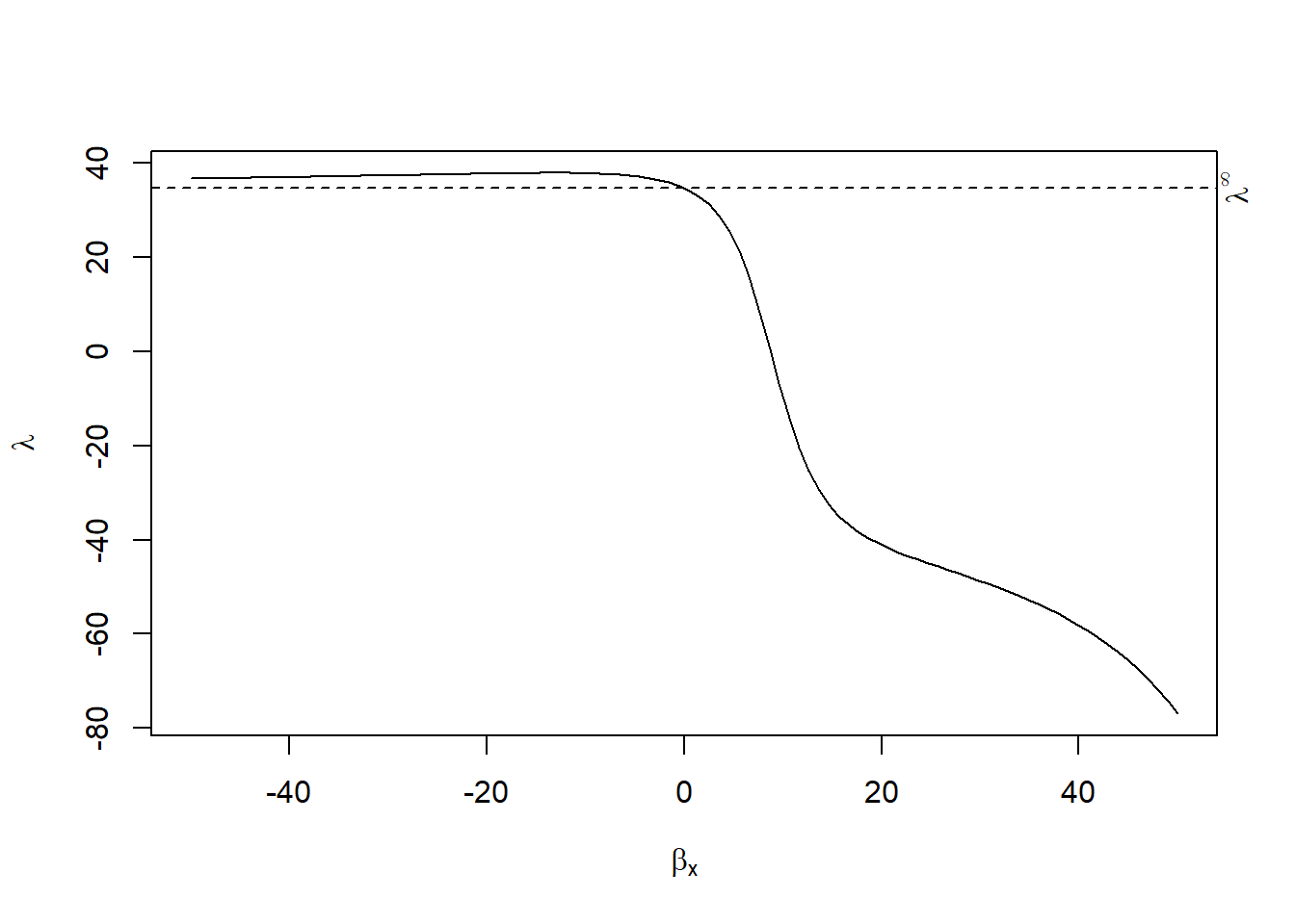
cor(Xi,ϵi)=λcor(Xi,Ciγ)
where λ∈(λl,λh)
Choice of λ
Strong assumption of no omitted variable bias (small
If λ=0, then cor(Xi,ϵi)=0
If λ=1, then cor(Xi,ϵi)=cor(Xi,Ciγ)
We typically examine λ∈(0,1)
# remotes::install_github("bvkrauth/rcr/r/rcrbounds")
library(rcrbounds)
# rcrbounds::install_rcrpy()
data("ChickWeight")

rcr_res <-
    rcrbounds::rcr(weight ~ Time |
                       Diet, ChickWeight, rc_range = c(0, 10))
rcr_res
#>
#> Call:
#> rcrbounds::rcr(formula = weight ~ Time | Diet, data = ChickWeight,
#>     rc_range = c(0, 10))
#>
#> Coefficients:
#>     rcInf effectInf       rc0   effectL   effectH
#> 34.676505 71.989336 34.741955  7.447713  8.750492
summary(rcr_res)
#>
#> Call:
#> rcrbounds::rcr(formula = weight ~ Time | Diet, data = ChickWeight,
#>     rc_range = c(0, 10))
#>
#> Coefficients:
#>            Estimate  Std. Error    t value      Pr(>|t|)
#> rcInf     34.676505  50.1295005  0.6917385  4.891016e-01
#> effectInf 71.989336 112.5711682  0.6395007  5.224973e-01
#> rc0       34.741955  58.7169195  0.5916856  5.540611e-01
#> effectL    7.447713   2.4276246  3.0679014  2.155677e-03
#> effectH    8.750492   0.2607671 33.5567355 7.180405e-247
#> ---
#> conservative confidence interval:
#>          2.5  %  97.5  %
#> effect 2.689656 9.261586

# hypothesis test for the coefficient
rcrbounds::effect_test(rcr_res, h0 = 0)
#> [1] 0.001234233
plot(rcr_res)