30.11 Assumptions
- Parallel Trends Assumption
- The treatment and control groups must follow parallel trends in the absence of treatment.
- Mathematically, this means the expected difference in potential outcomes remains constant over time:
E[Yit(0)|Di=1]−E[Yit(0)|Di=0] is constant over time.
- This assumption is crucial, as violations lead to biased estimates.
- Use DiD when:
- You have pre- and post-treatment data.
- You have clear treatment and control groups.
- Avoid DiD when:
- Treatment assignment is not random.
- There are confounders affecting trends differently.
- Testing Parallel Trends: Prior Parallel Trends Test.
- No Anticipation Effect (Pre-Treatment Exogeneity)
Individuals or groups should not change their behavior before the treatment is implemented in expectation of the treatment.
If units anticipate the treatment and adjust their behavior beforehand, it can introduce bias in the estimates.
- Exogenous Treatment Assignment
- Treatment should not be assigned based on potential outcomes.
- Ideally, assignment should be as good as random, conditional on observables.
- Stable Composition of Groups (No Attrition or Spillover)
- Treatment and control groups should remain stable over time.
- There should be no selective attrition (where individuals enter/leave due to treatment).
- No spillover effects: Control units should not be indirectly affected by treatment.
- No Simultaneous Confounding Events (Exogeneity of Shocks)
- There should be no other major shocks that affect treatment/control groups differently at the same time as treatment implementation.
Limitations and Common Issues
- Functional Form Dependence
- If the response to treatment is nonlinear, compare high- vs. low-intensity groups.
- Selection on (Time-Varying) Unobservables
- Use Rosenbaum Bounds to check the sensitivity of estimates to unobserved confounders.
- Long-Term Effects
- Parallel trends are more reliable in short time windows.
- Over long periods, other confounding factors may emerge.
- Heterogeneous Effects
- Treatment intensity (e.g., different doses) may vary across groups, leading to different effects.
- Ashenfelter’s Dip (Ashenfelter 1978)
- Participants in job training programs often experience earnings drops before enrolling, making them systematically different from nonparticipants.
- Fix: Compute long-run differences, excluding periods around treatment, to test for sustained impact (Proserpio and Zervas 2017a; J. J. Heckman, LaLonde, and Smith 1999; Jepsen, Troske, and Coomes 2014).
- Lagged Treatment Effects
- If effects are not immediate, using a lagged dependent variable Yit−1 may be more appropriate (Blundell and Bond 1998).
- Bias from Unobserved Factors Affecting Trends
- If external shocks influence treatment and control groups differently, this biases DiD estimates.
- Correlated Observations
- Standard errors should be clustered appropriately.
- Incidental Parameters Problem (Lancaster 2000)
- Always prefer individual and time fixed effects to reduce bias.
- Treatment Timing and Negative Weights
- If treatment timing varies across units, negative weights can arise in standard DiD estimators when treatment effects are heterogeneous (Athey and Imbens 2022; Borusyak, Jaravel, and Spiess 2024; Goodman-Bacon 2021).
- Fix: Use estimators from Callaway and Sant’Anna (2021) and Clément De Chaisemartin and d’Haultfoeuille (2020) (
didpackage). - If expecting lags and leads, see L. Sun and Abraham (2021).
- Treatment Effect Heterogeneity Across Groups
- If treatment effects vary across groups and interact with treatment variance, standard estimators may be invalid (Gibbons, Suárez Serrato, and Urbancic 2018).
- Endogenous Timing
If the timing of units can be influenced by strategic decisions in a DID analysis, an instrumental variable approach with a control function can be used to control for endogeneity in timing.
- Questionable Counterfactuals
In situations where the control units may not serve as a reliable counterfactual for the treated units, matching methods such as propensity score matching or generalized random forest can be utilized. Additional methods can be found in Matching Methods.
30.11.1 Prior Parallel Trends Test
The parallel trends assumption ensures that, absent treatment, the treated and control groups would have followed similar outcome trajectories. Testing this assumption involves visualization and statistical analysis.
Marcus and Sant’Anna (2021) discuss pre-trend testing in staggered DiD.
- Visual Inspection: Outcome Trends and Treatment Rollout
- Plot raw outcome trends for both groups before and after treatment.
- Use event-study plots to check for pre-trend violations and anticipation effects.
- Visualization tools like
ggplot2orpanelViewhelp illustrate treatment timing and trends.
- Event-Study Regressions
A formal test for pre-trends uses the event-study model:
Yit=α+K∑k=−Kβk1(T=k)+Xitγ+λi+δt+ϵit
where:
1(T=k) are time dummies for periods before and after treatment.
βk captures deviations in outcomes before treatment; these should be statistically indistinguishable from zero if parallel trends hold.
λi and δt are unit and time fixed effects.
Xit are optional covariates.
Violation of parallel trends occurs if pre-treatment coefficients (βk for k<0) are statistically significant.
- Statistical Test for Pre-Treatment Trend Differences
Using only pre-treatment data, estimate:
Y=αg+β1T+β2(T×G)+ϵ
where:
β2 measures differences in time trends between groups.
If β2=0, trends are parallel before treatment.
Considerations:
- Alternative functional forms (e.g., polynomials or nonlinear trends) can be tested.
- If β2≠0, potential explanations include:
- Large sample size driving statistical significance.
- Small deviations in one period disrupting an otherwise stable trend.
While time fixed effects can partially address violations of parallel trends (and are commonly used in modern research), they may also absorb part of the treatment effect, especially when treatment effects vary over time (Wolfers 2003).
Debate on Parallel Trends
- Levels vs. Trends: Kahn-Lang and Lang (2020) argue that similarity in levels is also crucial. If treatment and control groups start at different levels, why assume their trends will be the same?
- Solution:
- Plot time series for the treated and control groups.
- Use matched samples to improve comparability (Ryan et al. 2019) (useful when parallel trends assumption is questionable).
- If levels differ significantly, functional form assumptions become more critical and must be justified.
- Solution:
- Power of Pre-Trend Tests:
- Pre-trend tests often lack statistical power, making false negatives common (Roth 2022).
- See: PretrendsPower and pretrends (for adjustments).
- Outcome Transformations Matter:
- The parallel trends assumption is specific to both the transformation and units of the outcome variable (Roth and Sant’Anna 2023).
- Conduct falsification tests to check whether the assumption holds under different functional forms.
library(tidyverse)
library(fixest)
od <- causaldata::organ_donations %>%
    # Use only pre-treatment data
    filter(Quarter_Num <= 3) %>%
    # Treatment variable
    dplyr::mutate(California = State == 'California')

# use my package
causalverse::plot_par_trends(
    data = od,
    metrics_and_names = list("Rate" = "Rate"),
    treatment_status_var = "California",
    time_var = list(Quarter_Num = "Time"),
    display_CI = F
)
#> [[1]]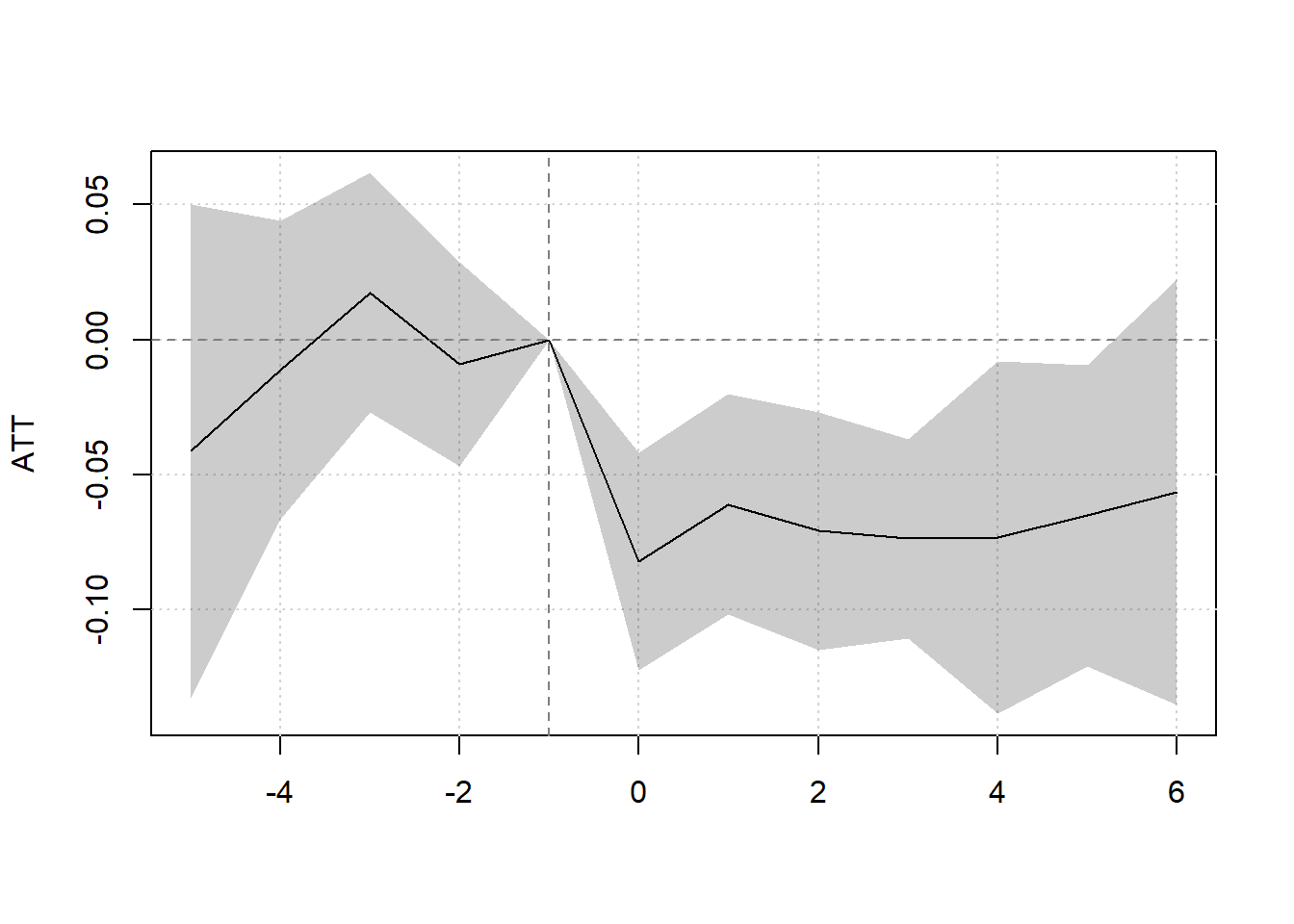
# do it manually
# always good but plot the dependent out
od |>
    # group by treatment status and time
    dplyr::group_by(California, Quarter) |>
    dplyr::summarize_all(mean) |>
    dplyr::ungroup() |>
    # view()

    ggplot2::ggplot(aes(x = Quarter_Num, y = Rate, color = California)) +
    ggplot2::geom_line() +
    causalverse::ama_theme()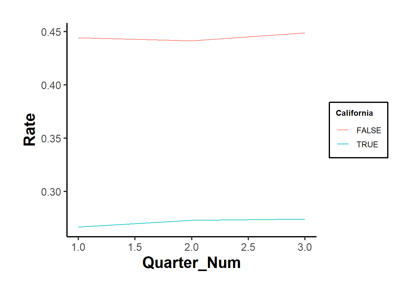
# but it's also important to use statistical test
prior_trend <- fixest::feols(Rate ~ i(Quarter_Num, California) |
                                 State + Quarter,
                             data = od)

fixest::coefplot(prior_trend, grid = F)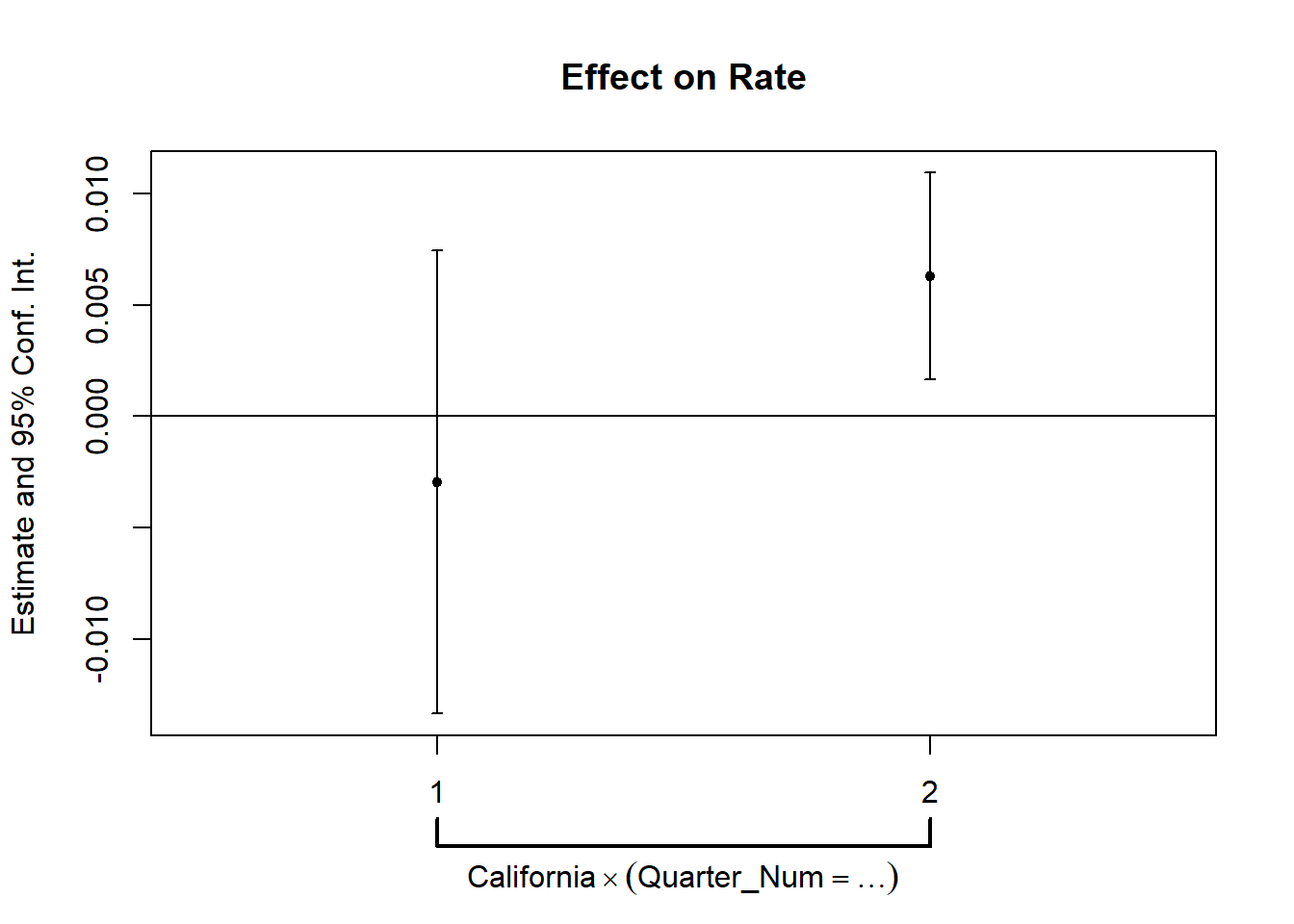
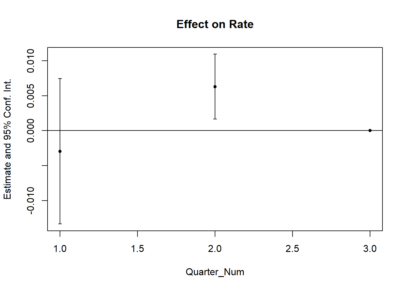
This is alarming since one of the periods is significantly different from 0, which means that our parallel trends assumption is not plausible.
In cases where the parallel trends assumption is questionable, researchers should consider methods for assessing and addressing potential violations. Some key approaches are discussed in Rambachan and Roth (2023):
Imposing Restrictions: Constrain how different the post-treatment violations of parallel trends can be relative to pre-treatment deviations.
Partial Identification: Rather than assuming a single causal effect, derive bounds on the ATT.
Sensitivity Analysis: Evaluate how sensitive the results are to potential deviations from parallel trends.
To implement these approaches, the HonestDiD package by Rambachan and Roth (2023) provides robust statistical tools:
# https://github.com/asheshrambachan/HonestDiD
# remotes::install_github("asheshrambachan/HonestDiD")
# library(HonestDiD)
Alternatively, Ban and Kedagni (2022) propose a method that incorporates pre-treatment covariates as an information set and makes an assumption about the selection bias in the post-treatment period. Specifically, they assume that the selection bias lies within the convex hull of all pre-treatment selection biases. Under this assumption:
They identify a set of possible ATT values.
With a stronger assumption on selection bias—grounded in policymakers’ perspectives—they can estimate a point estimate of ATT.
Another useful tool for assessing parallel trends is the pretrends package by Roth (2022), which provides formal pre-trend tests:
30.11.2 Placebo Test
A placebo test is a diagnostic tool used in Difference-in-Differences analysis to assess whether the estimated treatment effect is driven by pre-existing trends rather than the treatment itself. The idea is to estimate a treatment effect in a scenario where no actual treatment occurred. If a significant effect is found, it suggests that the parallel trends assumption may not hold, casting doubt on the validity of the causal inference.
Types of Placebo DiD Tests
- Group-Based Placebo Test
- Assign treatment to a group that was never actually treated and rerun the DiD model.
- If the estimated treatment effect is statistically significant, this suggests that differences between groups—not the treatment—are driving results.
- This test helps rule out the possibility that the estimated effect is an artifact of unobserved systematic differences.
A valid treatment effect should be consistent across different reasonable control groups. To assess this:
Rerun the DiD model using an alternative but comparable control group.
Compare the estimated treatment effects across multiple control groups.
If results vary significantly, this suggests that the choice of control group may be influencing the estimated effect, indicating potential selection bias or unobserved confounding.
- Time-Based Placebo Test
- Conduct DiD using only pre-treatment data, pretending that treatment occurred at an earlier period.
- A significant estimated treatment effect implies that differences in pre-existing trends—not treatment—are responsible for observed post-treatment effects.
- This test is particularly useful when concerns exist about unobserved shocks or anticipatory effects.
Random Reassignment of Treatment
- Keep the same treatment and control periods but randomly assign treatment to units that were not actually treated.
- If a significant DiD effect still emerges, it suggests the presence of biases, unobserved confounding, or systematic differences between groups that violate the parallel trends assumption.
Procedure for a Placebo Test
- Using Pre-Treatment Data Only
A robust placebo test often involves analyzing only pre-treatment periods to check whether spurious treatment effects appear. The procedure includes:
Restricting the sample to pre-treatment periods only.
Assigning a fake treatment period before the actual intervention.
Testing a sequence of placebo cutoffs over time to examine whether different assumed treatment timings yield significant effects.
Generating random treatment periods and using randomization inference to assess the sampling distribution of the placebo effect.
Estimating the DiD model using the fake post-treatment period (
post_time = 1).Interpretation: If the estimated treatment effect is statistically significant, this indicates that pre-existing trends (not treatment) might be influencing results, violating the parallel trends assumption.
- Using Control Groups for a Placebo Test
If multiple control groups are available, a placebo test can also be conducted by:
Dropping the actual treated group from the analysis.
Assigning one of the control groups as a fake treated group.
Estimating the DiD model and checking whether a significant effect is detected.
Interpretation:
If a placebo effect appears (i.e., the estimated treatment effect is significant), it suggests that even among control groups, systematic differences exist over time.
However, this result is not necessarily disqualifying. Some methods, such as Synthetic Control, explicitly model such differences while maintaining credibility.
# Load necessary libraries
library(tidyverse)
library(fixest)
library(ggplot2)
library(causaldata)

# Load the dataset
od <- causaldata::organ_donations %>%
    # Use only pre-treatment data
    dplyr::filter(Quarter_Num <= 3) %>%

    # Create fake (placebo) treatment variables
    dplyr::mutate(
        FakeTreat1 = as.integer(State == 'California' &
                                    Quarter %in% c('Q12011', 'Q22011')),
        FakeTreat2 = as.integer(State == 'California' &
                                    Quarter == 'Q22011')
    )

# Estimate the placebo effects using fixed effects regression
clfe1 <- fixest::feols(Rate ~ FakeTreat1 | State + Quarter, data = od)
clfe2 <- fixest::feols(Rate ~ FakeTreat2 | State + Quarter, data = od)

# Display the regression results
fixest::etable(clfe1, clfe2)
#>                           clfe1            clfe2
#> Dependent Var.:            Rate             Rate
#>
#> FakeTreat1      0.0061 (0.0051)
#> FakeTreat2                      -0.0017 (0.0028)
#> Fixed-Effects:  --------------- ----------------
#> State                       Yes              Yes
#> Quarter                     Yes              Yes
#> _______________ _______________ ________________
#> S.E.: Clustered       by: State        by: State
#> Observations                 81               81
#> R2                      0.99377          0.99376
#> Within R2               0.00192          0.00015
#> ---
#> Signif. codes: 0 '***' 0.001 '**' 0.01 '*' 0.05 '.' 0.1 ' ' 1

# Extract coefficients and confidence intervals
coef_df <- tibble(
    Model = c("FakeTreat1", "FakeTreat2"),
    Estimate = c(coef(clfe1)["FakeTreat1"], coef(clfe2)["FakeTreat2"]),
    SE = c(summary(clfe1)$coeftable["FakeTreat1", "Std. Error"],
           summary(clfe2)$coeftable["FakeTreat2", "Std. Error"]),
    Lower = Estimate - 1.96 * SE,
    Upper = Estimate + 1.96 * SE
)

# Plot the placebo effects
ggplot(coef_df, aes(x = Model, y = Estimate)) +
    geom_point(size = 3, color = "blue") +
    geom_errorbar(aes(ymin = Lower, ymax = Upper), width = 0.2, color = "blue") +
    geom_hline(yintercept = 0, linetype = "dashed", color = "red") +
    theme_minimal() +
    labs(
        title = "Placebo Treatment Effects",
        y = "Estimated Effect on Organ Donation Rate",
        x = "Placebo Treatment"
    )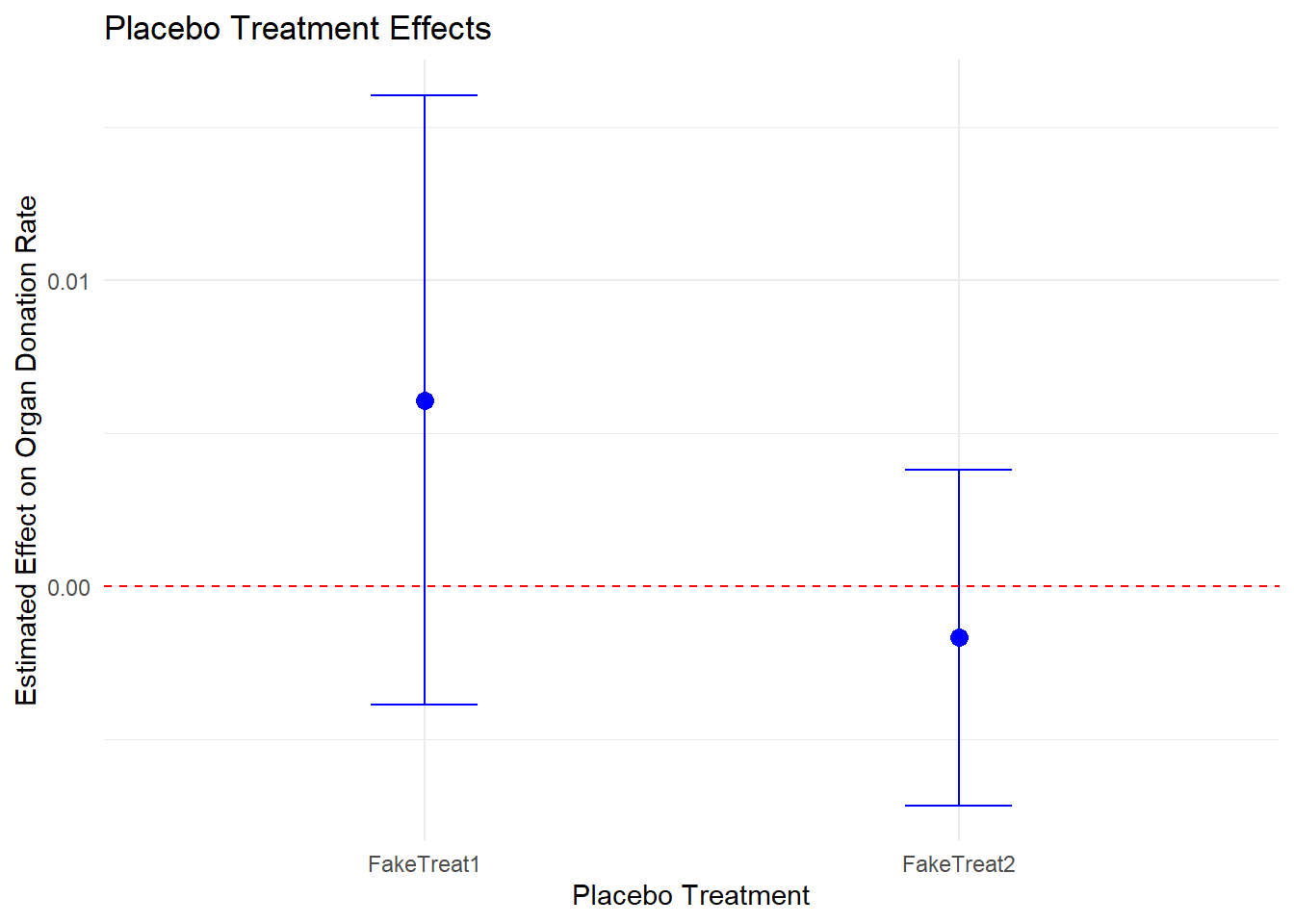
We would like the “supposed” DiD to be insignificant.