30.12 Nonlinear Difference-in-Differences

Traditional Difference-in-Differences methods typically rely on linear models with strong assumptions like constant treatment effects and homogeneous trends across treatment groups. These assumptions often fail in real-world data — especially when outcomes are binary, fractional, or counts, such as:

Employment status (binary),
Proportion of customers who churned (fraction),
Number of crimes in a neighborhood (count).

In these cases, the linear parallel trends assumption may be inappropriate. This chapter develops an advanced, flexible framework for nonlinear DiD estimation with staggered interventions (Wooldridge 2023).

30.12.1 Overview of Framework

We consider a panel dataset where units are observed over $T$ time periods. Units become treated at various times (staggered rollout), and the goal is to estimate Average Treatment Effect on the Treated (ATT) at different times.

Let $Y_{it}(g)$ denote the potential outcome at time $t$ if unit $i$ were first treated in period $g$ , with $g = q, \ldots, T$ or $g = \infty$ (never treated). Define the ATT for cohort $g$ at time $r \geq g$ as:

$\tau_{gr} = \mathbb{E}\left[Y_{ir}(g) - Y_{ir}(\infty) \mid D_g = 1\right]$

Here, $D_g = 1$ indicates that unit $i$ was first treated in period $g$ .

Rather than assuming linear conditional expectations of untreated outcomes, we posit a nonlinear conditional mean using a known, strictly increasing function $G(\cdot)$ :

$\mathbb{E}[Y_{it}(0) \mid D, X] = G\left( \alpha + \sum_{g=q}^{T} \beta_g D_g + X \kappa + \sum_{g=q}^{T} (D_g \cdot X)\eta_g + \gamma_t + X \pi_t \right)$

This formulation nests logistic and Poisson mean structures, and allows us to handle various limited dependent variables.

30.12.2 Assumptions

We require the following identification assumptions:

Conditional No Anticipation: $\mathbb{E}[Y_{it}(g) \mid D_g = 1, X] = \mathbb{E}[Y_{it}(\infty) \mid D_g = 1, X], \quad \forall t < g$
Conditional Index Parallel Trends: The untreated mean trends are parallel in a transformed index space: $\mathbb{E}[Y_{it}(\infty) \mid D, X] = G(\text{linear index in } D, X, t)$
- $G(\cdot)$ is a known, strictly increasing function (e.g., $\exp(\cdot)$ for Poisson)

These assumptions are weaker and more realistic than linear Parallel Trends, especially when outcomes are constrained.

30.12.3 Estimation Procedure

Step 1: Imputation Estimator

Estimate Parameters Using Untreated Observations Only:

Use all $(i,t)$ such that unit $i$ is untreated at $t$ (i.e., $W_{it} = 0$ ). Fit the nonlinear regression model: $Y_{it} = G\left(\alpha + \sum_g \beta_g D_g + X_i \kappa + D_g X_i \eta_g + \gamma_t + X_i \pi_t\right) + \varepsilon_{it}$

Impute Counterfactual Outcomes for Treated Observations:

For treated observations $(i,t)$ with $W_{it}=1$ , predict $\widehat{Y}_{it}(0)$ using the model from Step 1.

Compute ATT for Each Cohort $g$ and Time $r$ :

$\hat{\tau}_{gr} = \frac{1}{N_{gr}} \sum_{i: D_g=1} \left( Y_{ir} - \widehat{Y}_{ir}(0) \right)$

Step 2: Pooled QMLE Estimator (Equivalent When Using Canonical Link)

Fit Model Using All Observations:

Fit the pooled nonlinear model across all units and time: $Y_{it} = G\left(\alpha + \sum_g \beta_g D_g + X_i \kappa + D_g X_i \eta_g + \gamma_t + X_i \pi_t + \delta_r \cdot W_{it} + W_{it} X_i \xi \right) + \varepsilon_{it}$

Where:

$W_{it} = 1$ if unit $i$ is treated at time $t$
$W_{it} = 0$ otherwise

Estimate $\delta_r$ as the ATT for cohort $g$ in period $r$ :

$\delta_r$ is interpreted as an event-time ATT
This estimator is consistent when $G^{-1}(\cdot)$ is the canonical link (e.g., log link for Poisson)

Average Partial Effect (APE) for ATT:

$\hat{\tau}_{gr} = \frac{1}{N_g} \sum_{i: D_g=1} \left[ G\left( X_i\beta + \delta_r + \ldots \right) - G\left( X_i\beta + \ldots \right) \right]$

Canonical Links in Practice

Conditional Mean	LEF Density	Suitable For
$G(z) = z$	Normal	Any response
$G(z) = \exp(z)$	Poisson	Nonnegative/counts, no natural upper bound
$G(z) = \text{logit}^{-1}(z)$	Binomial	Nonnegative, known upper bound
$G(z) = \text{logit}^{-1}(z)$	Bernoulli	Binary or fractional responses

30.12.4 Inference

Standard errors can be obtained via the delta method or bootstrap
Cluster-robust standard errors by unit are preferred
When using QMLE, the estimates are valid under correct mean specification, regardless of higher moments

When Do Imputation and Pooled Methods Match?

They are numerically identical when:
- Estimating with the canonical link function
- Model is correctly specified
- Same data used for both (i.e., W_it = 0 and pooled)

30.12.5 Application Using `etwfe`

The etwfe package provides a unified, user-friendly interface for estimating staggered treatment effects using generalized linear models. It is particularly well-suited for nonlinear outcomes, such as binary, fractional, or count data.

We’ll now demonstrate how to apply etwfe to estimate Average Treatment Effect on the Treated (ATT) under a nonlinear DiD framework using a Poisson model. This aligns with the exponential conditional mean assumption discussed earlier.

Install and load packages

# --- 1) Load packages ---
# install.packages("fixest")
# install.packages("marginaleffects")
# install.packages("etwfe")
# install.packages("ggplot2")
# install.packages("modelsummary")

library(etwfe)
library(fixest)
library(marginaleffects)
library(ggplot2)
library(modelsummary)
set.seed(12345)

Simulate a known data-generating process

Imagine a multi-period business panel where each “unit” is a regional store or branch of a large retail chain. Half of these stores eventually receive a new marketing analytics platform at some known time, which in principle changes their performance metric (e.g., weekly log sales). The other half never receive the platform, functioning as a “never-treated” control group.

We have $N=200$ stores (half eventually treated, half never treated).
Each store is observed over $T=10$ time periods (e.g., quarters or years).
The true “treatment effect on the treated” is constant at $\delta = -0.05$ for all post-treatment times. (Interpretation: the new marketing platform reduced log-sales by about 5 percent, though in real life one might expect a positive effect!)
Some stores are “staggered” in the sense that they adopt in different periods. We’ll randomly draw their adoption date from $\{4,5,6\}$ . Others never adopt at all.
We include store-level intercepts, time intercepts, and idiosyncratic noise to make it more realistic.

# --- 2) Simulate Data ---
N <- 200   # number of stores
T <- 10    # number of time periods
id   <- rep(1:N, each = T)
time <- rep(1:T, times = N)

# Mark half of them as eventually treated, half never
treated_ids <- sample(1:N, size = N/2, replace = FALSE)
is_treated  <- id %in% treated_ids

# Among the treated, pick an adoption time 4,5, or 6 at random
adopt_time_vec <- sample(c(4,5,6), size = length(treated_ids), replace = TRUE)
adopt_time     <- rep(0, N) # 0 means "never"
adopt_time[treated_ids] <- adopt_time_vec

# Store effects, time effects, control variable, noise
alpha_i <- rnorm(N, mean = 2, sd = 0.5)[id]
gamma_t <- rnorm(T, mean = 0, sd = 0.2)[time]
xvar    <- rnorm(N*T, mean = 1, sd = 0.3)
beta    <- 0.10
noise   <- rnorm(N*T, mean = 0, sd = 0.1)

# True treatment effect = -0.05 for time >= adopt_time
true_ATT <- -0.05
D_it     <- as.numeric((adopt_time[id] != 0) & (time >= adopt_time[id]))

# Final outcome in logs:
y <- alpha_i + gamma_t + beta*xvar + true_ATT*D_it + noise

# Put it all in a data frame
simdat <- data.frame(
    id         = id,
    time       = time,
    adopt_time = adopt_time[id],
    treat      = D_it,
    xvar       = xvar,
    logY       = y
)

head(simdat)
#>   id time adopt_time treat      xvar     logY
#> 1  1    1          6     0 1.4024608 1.317343
#> 2  1    2          6     0 0.5226395 2.273805
#> 3  1    3          6     0 1.3357914 1.517705
#> 4  1    4          6     0 1.2101680 1.759481
#> 5  1    5          6     0 0.9953143 1.771928
#> 6  1    6          6     1 0.8893066 1.439206

In this business setting, you can imagine that logY is the natural log of revenue, sales, or another KPI, and xvar is a log of local population, number of competitor stores in the region, or similar.

Estimate with etwfe

We want to test whether the new marketing analytics platform has changed the log outcome. We will use etwfe:

fml = logY ~ xvar says that logY is the outcome, xvar is a control.
tvar = time is the time variable.
gvar = adopt_time is the group/cohort variable (the “first treatment time” or 0 if never).
vcov = ~id clusters standard errors at the store level.
cgroup = "never": We specify that the never-treated units form our comparison group. This ensures we can see pre-treatment and post-treatment dynamic effects in an event-study plot.

# --- 3) Estimate with etwfe ---
mod <- etwfe(
    fml    = logY ~ xvar,
    tvar   = time,
    gvar   = adopt_time,
    data   = simdat,
    vcov   = ~id,
    cgroup = "never"  # so that never-treated are the baseline
)

Nothing fancy will appear in the raw coefficient list because it’s fully “saturated” with interactions. The real prize is in the aggregated treatment effects, which we’ll obtain next.

Recover the average treatment effect on the treated (ATT)

Here’s a single-number estimate of the overall average effect on the treated, across all times and cohorts:

# --- 4) Single-number ATT ---
ATT_est <- emfx(mod, type = "simple")
print(ATT_est)
#> 
#>  .Dtreat Estimate Std. Error     z Pr(>|z|)    S  2.5 %  97.5 %
#>     TRUE  -0.0707     0.0178 -3.97   <0.001 13.8 -0.106 -0.0358
#> 
#> Term: .Dtreat
#> Type:  response 
#> Comparison: TRUE - FALSE

You should see an estimate near the true $-0.05$ .

Recover an event-study pattern of dynamic effects

To check pre- and post-treatment dynamics, we ask for an event study via type = "event". This shows how the outcome evolves around the adoption time. Negative “event” values correspond to pre-treatment, while nonnegative “event” values are post-treatment.

# --- 5) Event-study estimates ---
mod_es <- emfx(mod, type = "event")
print(mod_es)
#> 
#>  event Estimate Std. Error      z Pr(>|z|)    S   2.5 %   97.5 %
#>     -5 -0.04132     0.0467 -0.885  0.37628  1.4 -0.1329  0.05022
#>     -4 -0.01120     0.0282 -0.396  0.69180  0.5 -0.0666  0.04416
#>     -3  0.01747     0.0226  0.772  0.43999  1.2 -0.0269  0.06180
#>     -2 -0.00912     0.0193 -0.472  0.63686  0.7 -0.0470  0.02873
#>     -1  0.00000         NA     NA       NA   NA      NA       NA
#>      0 -0.08223     0.0206 -3.995  < 0.001 13.9 -0.1226 -0.04188
#>      1 -0.06108     0.0209 -2.926  0.00344  8.2 -0.1020 -0.02016
#>      2 -0.07094     0.0225 -3.159  0.00158  9.3 -0.1150 -0.02692
#>      3 -0.07383     0.0189 -3.906  < 0.001 13.4 -0.1109 -0.03679
#>      4 -0.07330     0.0334 -2.196  0.02808  5.2 -0.1387 -0.00788
#>      5 -0.06527     0.0285 -2.294  0.02178  5.5 -0.1210 -0.00951
#>      6 -0.05661     0.0402 -1.407  0.15953  2.6 -0.1355  0.02227
#> 
#> Term: .Dtreat
#> Type:  response 
#> Comparison: TRUE - FALSE

By default, this will return events from (roughly) the earliest pre-treatment period up to the maximum possible post-treatment period in your data, using never-treated as the comparison group.
Inspect the estimates and confidence intervals. Ideally, pre-treatment estimates should be near 0, and post-treatment estimates near $-0.05$ .

Plot the estimated event-study vs. the true effect

In a business or marketing study, a useful final step is a chart showing the point estimates (with confidence bands) plus the known true effect as a reference.

Construct the “true” dynamic effect curve

Pre-treatment periods: effect = 0
Post-treatment periods: effect = $\delta=-0.05$

Below we will:

Extract the estimated event effects from mod_es.
Build a reference dataset with the same event times.
Plot both on the same figure.

# --- 6) Plot results vs. known effect ---
est_df <- as.data.frame(mod_es)

range_of_event <- range(est_df$event)
event_breaks   <- seq(range_of_event[1], range_of_event[2], by = 1)
true_fun <- function(e) ifelse(e < 0, 0, -0.05)
event_grid <- seq(range_of_event[1], range_of_event[2], by = 1)
true_df <- data.frame(
    event       = event_grid,
    true_effect = sapply(event_grid, true_fun)
)

ggplot() +
    # Confidence interval ribbon (put it first so it's behind everything)
    geom_ribbon(
        data = est_df,
        aes(x = event, ymin = conf.low, ymax = conf.high),
        fill = "grey60",   # light gray fill
        alpha = 0.3
    ) +
    # Estimated effect line
    geom_line(
        data = est_df,
        aes(x = event, y = estimate),
        color = "black",
        size = 1
    ) +
    # Estimated effect points
    geom_point(
        data = est_df,
        aes(x = event, y = estimate),
        color = "black",
        size = 2
    ) +
    # Known true effect (dashed red line)
    geom_line(
        data = true_df,
        aes(x = event, y = true_effect),
        color = "red",
        linetype = "dashed",
        size = 1
    ) +
    # Horizontal zero line
    geom_hline(yintercept = 0, linetype = "dotted") +
    # Vertical line at event = 0 for clarity
    geom_vline(xintercept = 0, color = "gray40", linetype = "dashed") +
    # Make sure x-axis breaks are integers
    scale_x_continuous(breaks = event_breaks) +
    labs(
        title = "Event-Study Plot vs. Known True Effect",
        subtitle = "Business simulation with new marketing platform adoption",
        x = "Event time (periods relative to adoption)",
        y = "Effect on log-outcome (ATT)",
        caption = "Dashed red line = known true effect; Shaded area = 95% CI"
    ) +
    causalverse::ama_theme()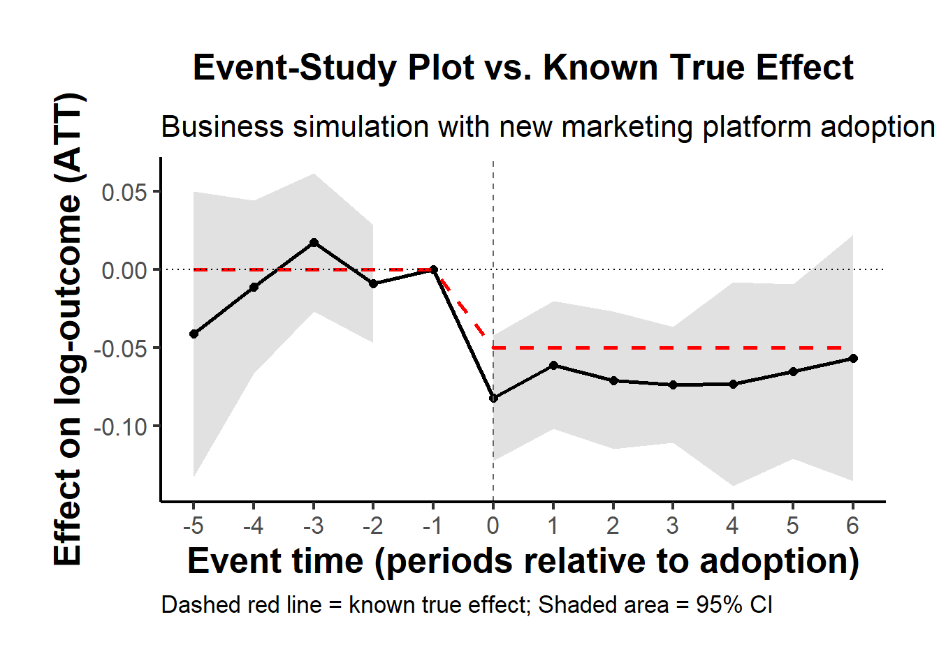

Solid line and shaded region: the ETWFE point estimates and their 95% confidence intervals, for each event time relative to adoption.
Dashed red line: the true effect that we built into the DGP.

If the estimation works well (and your sample is big enough), the estimated event-study effects should hover near the dashed red line post-treatment, and near zero pre-treatment.

Double-check in a regression table (optional)

If you like to see a clean numeric summary of the dynamic estimates by period, you can pipe your event-study object into modelsummary:

# --- 7) Optional table for dynamic estimates ---
modelsummary(
    list("Event-Study" = mod_es),
    shape     = term + statistic ~ model + event,
    gof_map   = NA,
    coef_map  = c(".Dtreat" = "ATT"),
    title     = "ETWFE Event-Study by Relative Adoption Period",
    notes     = "Std. errors are clustered by store ID"
)

ETWFE Event-Study by Relative Adoption Period
	Event-Study
	-5	-4	-3	-2	-1	0	1	2	3	4	5	6
Std. errors are clustered by store ID
ATT	-0.041	-0.011	0.017	-0.009	0.000	-0.082	-0.061	-0.071	-0.074	-0.073	-0.065	-0.057
	(0.047)	(0.028)	(0.023)	(0.019)		(0.021)	(0.021)	(0.022)	(0.019)	(0.033)	(0.028)	(0.040)

References

———. 2023. “Simple Approaches to Nonlinear Difference-in-Differences with Panel Data.” The Econometrics Journal 26 (3): C31–66.