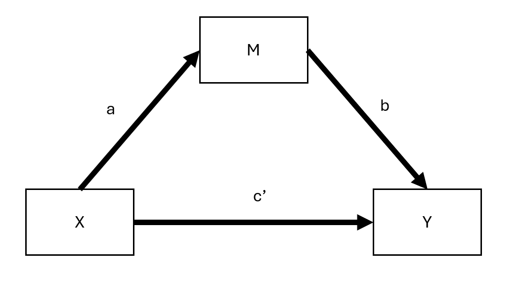
42.1 Traditional Approach
Baron and Kenny (1986) is outdated because of step 1, but we could still see the original idea.
3 regressions
Step 1: \(X \to Y\)
Step 2: \(X \to M\)
Step 3: \(X + M \to Y\)
where
\(X\) = independent (causal) variable
\(Y\) = dependent (outcome) variable
\(M\) = mediating variable
Note: Originally, the first path from \(X \to Y\) suggested by (Baron and Kenny 1986) needs to be significant. But there are cases in which you could have indirect of \(X\) on \(Y\) without significant direct effect of \(X\) on \(Y\) (e.g., when the effect is absorbed into M, or there are two counteracting effects \(M_1, M_2\) that cancel out each other effect).

where \(c\) is the total effect

where
\(c'\) = direct effect (effect of \(X\) on \(Y\) after accounting for the indirect path)
\(ab\) = indirect effect
Hence,
\[ \begin{aligned} \text{total effect} &= \text{direct effect} + \text{indirect effect} \\ c &= c' + ab \end{aligned} \]
However, this simple equation does not only hold in cases of
- Models with latent variables
- Logistic models (only approximately). Hence, you can only calculate \(c\) as the total effect of \(c' + ab\)
- Multi-level models (Bauer, Preacher, and Gil 2006)
To measure mediation (i.e., indirect effect),
- \(1 - \frac{c'}{c}\) highly unstable (D. P. MacKinnon, Warsi, and Dwyer 1995), especially in cases that \(c\) is small (not re* recommended)
- Product method: \(a\times b\)
- Difference method: \(c- c'\)
For linear models, we have the following assumptions:
No unmeasured confound between \(X-Y\), \(X-M\) and \(M-Y\) relationships.
\(X \not\rightarrow C\) where \(C\) is a confounder between \(M-Y\) relationship
Reliability: No errors in measurement of \(M\) (also known as reliability assumption) (can consider errors-in-variables models)
Mathematically,
\[ Y = b_0 + b_1 X + \epsilon \]
\(b_1\) does not need to be significant.
- We examine the effect of \(X\) on \(M\). This step requires that there is a significant effect of \(X\) on \(M\) to continue with the analysis
Mathematically,
\[ M = b_0 + b_2 X + \epsilon \]
where \(b_2\) needs to be significant.
- In this step, we want to the effect of \(M\) on \(Y\) “absorbs” most of the direct effect of \(X\) on \(Y\) (or at least makes the effect smaller).
Mathematically,
\[ Y = b_0 + b_4 X + b_3 M + \epsilon \]
\(b_4\) needs to be either smaller or insignificant.
| The effect of \(X\) on \(Y\) | then, \(M\) … mediates between \(X\) and \(Y\) |
|---|---|
| completely disappear (\(b_4\) insignificant) | Fully (i.e., full mediation) |
| partially disappear (\(b_4 < b_1\) in step 1) | Partially (i.e., partial mediation) |
- Examine the mediation effect (i.e., whether it is significant)
Bootstrapping Shrout and Bolger (2002) (preferable)
Notes:
Proximal mediation (\(a > b\)) can lead to multicollinearity and reduce statistical power, whereas distal mediation (\(b > a\)) is preferred for maximizing test power.
The ideal balance for maximizing power in mediation analysis involves slightly distal mediators (i.e., path \(b\) is somewhat larger than path \(a\)) (Hoyle 1999).
Tests for direct effects (c and c') have lower power compared to the indirect effect (ab), making it possible for ab to be significant while c is not, even in cases where there seems to be complete mediation but no statistical evidence of a direct cause-effect relationship between X and Y without considering M (Kenny and Judd 2014).
The testing of \(ab\) offers a power advantage over \(c’\) because it effectively combines two tests. However, claims of complete mediation based solely on the non-significance of \(c’\) should be approached with caution, emphasizing the need for sufficient sample size and power, especially in assessing partial mediation. Or one should never make complete mediation claim (Hayes and Scharkow 2013)
42.1.1 Assumptions
42.1.1.1 Direction
Quick fix but not convincing: Measure \(X\) before \(M\) and \(Y\) to prevent \(M\) or \(Y\) causing \(X\); measure \(M\) before \(Y\) to avoid \(Y\) causing \(M\).
\(Y\) may cause \(M\) in a feedback model.
Assuming \(c' =0\) (full mediation) allows for estimating models with reciprocal causal effects between \(M\) and \(Y\) via IV estimation.
E. R. Smith (1982) proposes treating both \(M\) and \(Y\) as outcomes with potential to mediate each other, requiring distinct instrumental variables for each that do not affect the other.
42.1.1.2 Interaction
When M interact with X to affect Y, M is both a mediator and a mediator (Baron and Kenny 1986).
Interaction between \(XM\) should always be estimated.
For the interpretation of this interaction, see (T. VanderWeele 2015)
42.1.1.3 Reliability
When mediator contains measurement errors, \(b, c'\) are biased. Possible fix: mediator = latent variable (but loss of power) (Ledgerwood and Shrout 2011)
\(b\) is attenuated (closer to 0)
\(c'\) is
overestimated when \(ab >0\)
underestiamted when \(ab<0\)
When treatment contains measurement errors, \(a,b\) are biased
\(a\) is attenuated
\(b\) is
overestimated when \(ac'>0\)
underestimated when \(ac' <0\)
When outcome contains measurement errors,
If unstandardized, no bias
If standardized, attenuation bias
42.1.1.4 Confounding
Omitted variable bias can happen to any pair of relationships
To deal with this problem, one can either use
42.1.1.4.1 Design Strategies
Randomization of treatment variable. If possible, also mediator
Control for the confounder (but still only for measureable observables)
42.1.1.4.2 Statistical Strategies
Instrumental variable on treatment
- Specifically for confounder affecting the \(M-Y\) pair, front-door adjustment is possible when there is a variable that completely mediates the effect of the mediator on the outcome and is unaffected by the confounder.
Weighting methods (e.g., inverse propensity) See Heiss for R code
- Need strong ignorability assumption (i.e.., all confounders are included and measured without error (Westfall and Yarkoni 2016)). Not fixable, but can be examined with robustness checks.
42.1.2 Indirect Effect Tests
42.1.2.1 Sobel Test
developed by Sobel (1982)
also known as the delta method
not recommend because it assumes the indirect effect \(b\) has a normal distribution when it’s not (D. P. MacKinnon, Warsi, and Dwyer 1995).
Mediation can occur even if direct and indirect effects oppose each other, termed “inconsistent mediation” (D. P. MacKinnon, Fairchild, and Fritz 2007). This is when the mediator acts as a suppressor variable.
Standard Error
\[ \sqrt{\hat{b}^2 s_{\hat{a}} + \hat{a}^2 s_{b}^2} \]
The test of the indirect effect is
\[ z = \frac{\hat{ab}}{\sqrt{\hat{b}^2 s_{\hat{a}} + \hat{a}^2 s_{b}^2}} \]
Disadvantages
Assume \(a\) and \(b\) are independent.
Assume \(ab\) is normally distributed.
Does not work well for small sample sizes.
Power of the test is low and the test is conservative as compared to Bootstrapping.
42.1.2.2 Joint Significance Test
Effective for determining if the indirect effect is nonzero (by testing whether \(a\) and \(b\) are both statistically significant), assumes \(a \perp b\).
It’s recommended to use it with other tests and has similar performance to a Bootstrapping test (Hayes and Scharkow 2013).
The test’s accuracy can be affected by heteroscedasticity (Fossum and Montoya 2023) but not by non-normality.
Although helpful in computing power for the test of the indirect effect, it doesn’t provide a confidence interval for the effect.
42.1.2.3 Bootstrapping
First used by Bollen and Stine (1990)
It allows for the calculation of confidence intervals, p-values, etc.
It does not require \(a \perp b\) and corrects for bias in the bootstrapped distribution.
It can handle non-normality (in the sampling distribution of the indirect effect), complex models, and small samples.
Concerns exist about the bias-corrected bootstrapping being too liberal (Fritz, Taylor, and MacKinnon 2012). Hence, current recommendations favor percentile bootstrap without bias correction for better Type I error rates (Tibbe and Montoya 2022).
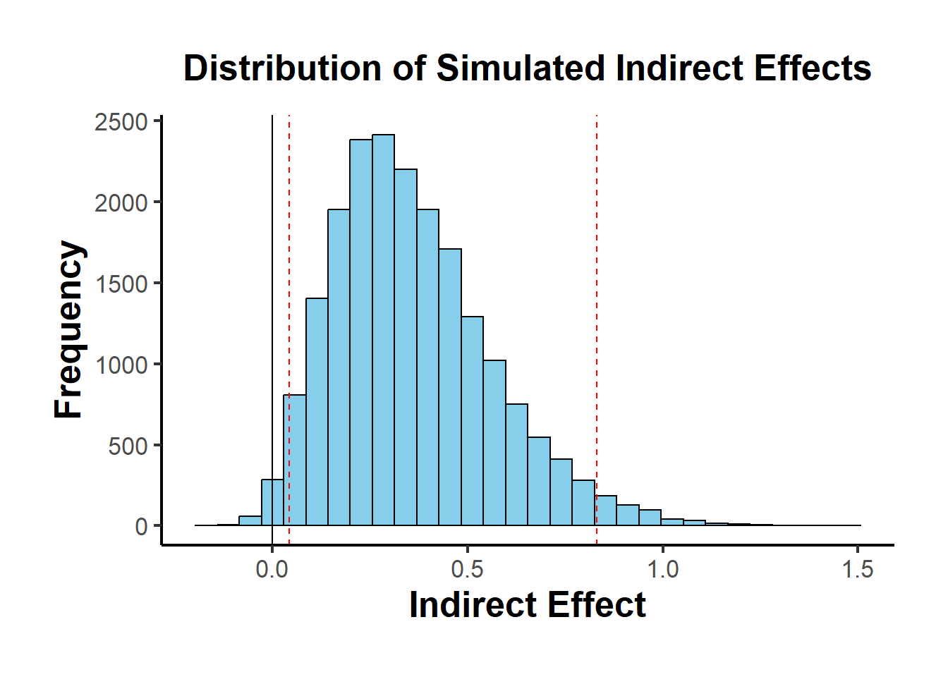
A special case of bootstrapping is a proposed by where you don’t need access to raw data to generate resampling, you only need \(a, b, var(a), var(b), cov(a,b)\) (which can be taken from lots of primary studies)
result <-
    causalverse::med_ind(
        a = 0.5,
        b = 0.7,
        var_a = 0.04,
        var_b = 0.05,
        cov_ab = 0.01
    )
result$plot
42.1.2.3.1 With Instrument
library(DiagrammeR)
grViz("
digraph {
  graph []
  node [shape = plaintext]
    X [label = 'Treatment']
    Y [label = 'Outcome']
  edge [minlen = 2]
    X->Y
  { rank = same; X; Y }
}
")

grViz("
digraph {
  graph []
  node [shape = plaintext]
    X [label ='Treatment', shape = box]
    Y [label ='Outcome', shape = box]
    M [label ='Mediator', shape = box]
    IV [label ='Instrument', shape = box]
  edge [minlen = 2]
    IV->X
    X->M
    M->Y
    X->Y
  { rank = same; X; Y; M }
}
")library(mediation)
data("boundsdata")
library(fixest)
# Total Effect
out1 <- feols(out ~ ttt, data = boundsdata)
# Indirect Effect
out2 <- feols(med ~ ttt, data = boundsdata)
# Direct and Indirect Effect
out3 <- feols(out ~ med + ttt, data = boundsdata)
# Proportion Test
# To what extent is the effect of the treatment mediated by the mediator?
coef(out2)['ttt'] * coef(out3)['med'] / coef(out1)['ttt'] * 100
#> ttt
#> 68.63609
# Sobel Test
bda::mediation.test(boundsdata$med, boundsdata$ttt, boundsdata$out) |>
tibble::rownames_to_column() |>
causalverse::nice_tab(2)
#> rowname Sobel Aroian Goodman
#> 1 z.value 4.05 4.03 4.07
#> 2 p.value 0.00 0.00 0.00# Mediation Analysis using boot
library(boot)
set.seed(1)
mediation_fn <- function(data, i){
# sample the dataset
df <- data[i,]
a_path <- feols(med ~ ttt, data = df)
a <- coef(a_path)['ttt']
b_path <- feols(out ~ med + ttt, data = df)
b <- coef(b_path)['med']
cp <- coef(b_path)['ttt']
# indirect effect
ind_ef <- a*b
total_ef <- a*b + cp
return(c(ind_ef, total_ef))
}
boot_med <- boot(boundsdata, mediation_fn, R = 100, parallel = "multicore", ncpus = 2)
boot_med
#>
#> ORDINARY NONPARAMETRIC BOOTSTRAP
#>
#>
#> Call:
#> boot(data = boundsdata, statistic = mediation_fn, R = 100, parallel = "multicore",
#> ncpus = 2)
#>
#>
#> Bootstrap Statistics :
#> original bias std. error
#> t1* 0.04112035 0.0006346725 0.009539903
#> t2* 0.05991068 -0.0004462572 0.029556611
summary(boot_med) |>
causalverse::nice_tab()
#> R original bootBias bootSE bootMed
#> 1 100 0.04 0 0.01 0.04
#> 2 100 0.06 0 0.03 0.06
# confidence intervals (percentile is always recommended)
boot.ci(boot_med, type = c("norm", "perc"))
#> BOOTSTRAP CONFIDENCE INTERVAL CALCULATIONS
#> Based on 100 bootstrap replicates
#>
#> CALL :
#> boot.ci(boot.out = boot_med, type = c("norm", "perc"))
#>
#> Intervals :
#> Level Normal Percentile
#> 95% ( 0.0218, 0.0592 ) ( 0.0249, 0.0623 )
#> Calculations and Intervals on Original Scale
#> Some percentile intervals may be unstable
# point estimates (Indirect, and Total Effects)
colMeans(boot_med$t)
#> [1] 0.04175502 0.05946442Alternatively, one can use the robmed package
Power test or use app