29.9 Application
Packages:
eventstudiesererEventStudyAbnormalReturnsPerformanceAnalytics
In practice, people usually sort portfolio because they are not sure whether the FF model is specified correctly.
Steps:
- Sort all returns in CRSP into 10 deciles based on size.
- In each decile, sort returns into 10 decides based on BM
- Get the average return of the 100 portfolios for each period (i.e., expected returns of stocks given decile - characteristics)
- For each stock in the event study: Compare the return of the stock to the corresponding portfolio based on size and BM.
Notes:
Sorting produces outcomes that are often more conservative (e.g., FF abnormal returns can be greater than those that used sorting).
If the results change when we do B/M first then size or vice versa, then the results are not robust (this extends to more than just two characteristics - e.g., momentum).
Examples:
Forestry:
(Mei and Sun 2008) M&A on financial performance (forest product)
(C. Sun and Liao 2011) litigation on firm values
library(erer)

# example by the package's author
data(daEsa)
hh <- evReturn(
    y = daEsa,       # dataset
    firm = "wpp",    # firm name
    y.date = "date", # date in y
    index = "sp500", # index
    est.win = 250,   # estimation window wedith in days
    digits = 3,
    event.date = 19990505, # firm event dates
    event.win = 5          # one-side event window wdith in days (default = 3, where 3 before + 1 event date + 3 days after = 7 days)
)
hh; plot(hh)
#>
#> === Regression coefficients by firm =========
#>   N firm event.date alpha.c alpha.e alpha.t alpha.p alpha.s beta.c beta.e
#> 1 1  wpp   19990505  -0.135   0.170  -0.795   0.428          0.665  0.123
#>   beta.t beta.p beta.s
#> 1  5.419  0.000    ***
#>
#> === Abnormal returns by date ================
#>    day Ait.wpp    HNt
#> 1   -5   4.564  4.564
#> 2   -4   0.534  5.098
#> 3   -3  -1.707  3.391
#> 4   -2   2.582  5.973
#> 5   -1  -0.942  5.031
#> 6    0  -3.247  1.784
#> 7    1  -0.646  1.138
#> 8    2  -2.071 -0.933
#> 9    3   0.368 -0.565
#> 10   4   4.141  3.576
#> 11   5   0.861  4.437
#>
#> === Average abnormal returns across firms ===
#>      name estimate error t.value p.value sig
#> 1 CiT.wpp    4.437 8.888   0.499   0.618
#> 2     GNT    4.437 8.888   0.499   0.618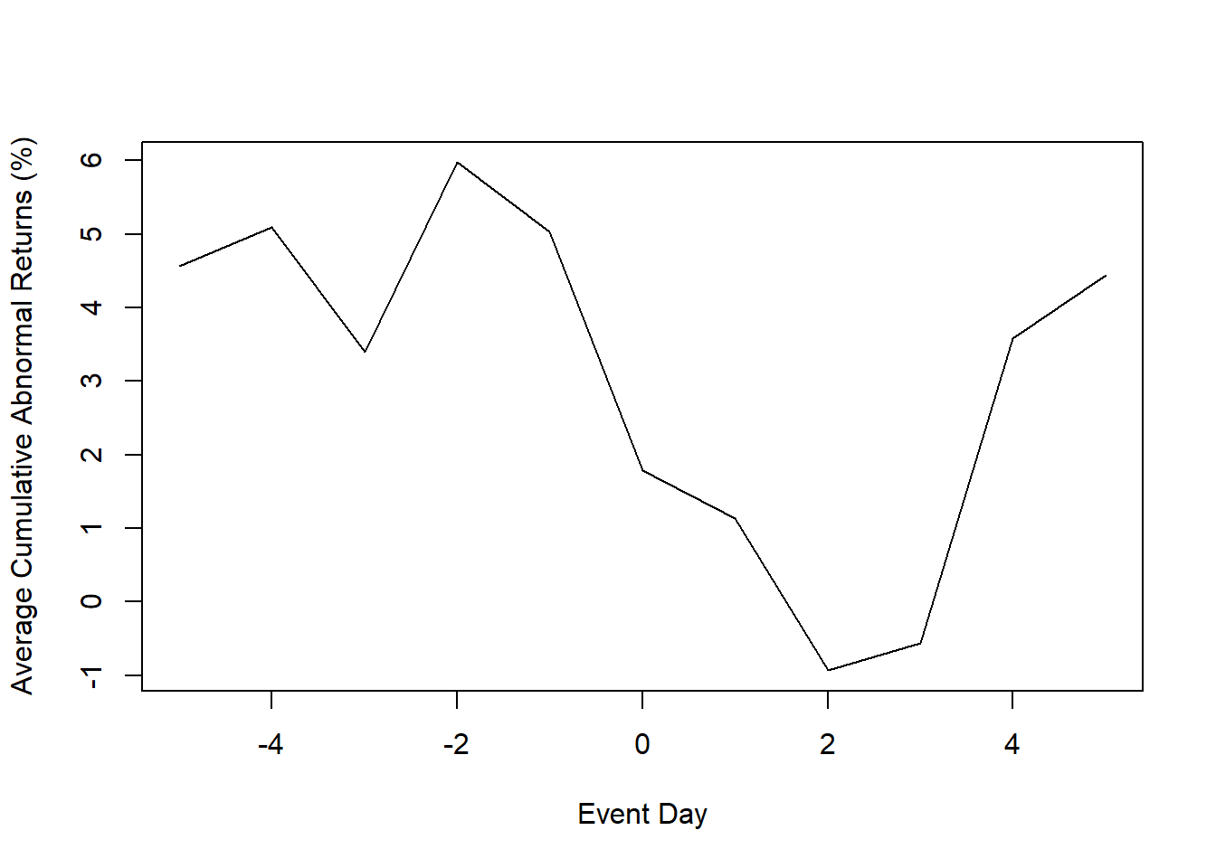
Example by Ana Julia Akaishi Padula, Pedro Albuquerque (posted on LAMFO)
Example in AbnormalReturns package
29.9.1 Eventus
2 types of output:
Using different estimation methods (e.g., market model to calendar-time approach)
Does not include event-specific returns. Hence, no regression later to determine variables that can affect abnormal stock returns.
Cross-sectional Analysis of Eventus: Event-specific abnormal returns (using monthly or data data) for cross-sectional analysis (under Cross-Sectional Analysis section)
- Since it has the stock-specific abnormal returns, we can do regression on CARs later. But it only gives market-adjusted model. However, according to (A. Sorescu, Warren, and Ertekin 2017), they advocate for the use of market-adjusted model for the short-term only, and reserve the FF4 for the longer-term event studies using monthly daily.
29.9.1.1 Basic Event Study
- Input a text file contains a firm identifier (e.g., PERMNO, CUSIP) and the event date
- Choose market indices: equally weighted and the value weighted index (i.e., weighted by their market capitalization). And check Fama-French and Carhart factors.
- Estimation options
Estimation period:
ESTLEN = 100is the convention so that the estimation is not impacted by outliers.Use “autodate” options: the first trading after the event date is used if the event falls on a weekend or holiday
- Abnormal returns window: depends on the specific event
- Choose test: either parametric (including Patell Standardized Residual (PSR)) or non-parametric
29.9.1.2 Cross-sectional Analysis of Eventus
Similar to the Basic Event Study, but now you can have event-specific abnormal returns.
29.9.2 Evenstudies
This package does not use the Fama-French model, only the market models.
This example is by the author of the package
library(eventstudies)
# firm and date data
data("SplitDates")
head(SplitDates)

# stock price data
data("StockPriceReturns")
head(StockPriceReturns)
class(StockPriceReturns)

es <-
    eventstudy(
        firm.returns = StockPriceReturns,
        event.list = SplitDates,
        event.window = 5,
        type = "None",
        to.remap = TRUE,
        remap = "cumsum",
        inference = TRUE,
        inference.strategy = "bootstrap"
    )

plot(es)
29.9.3 EventStudy
You have to pay for the API key. (It’s $10/month).
Example by the authors of the package
Data Prep
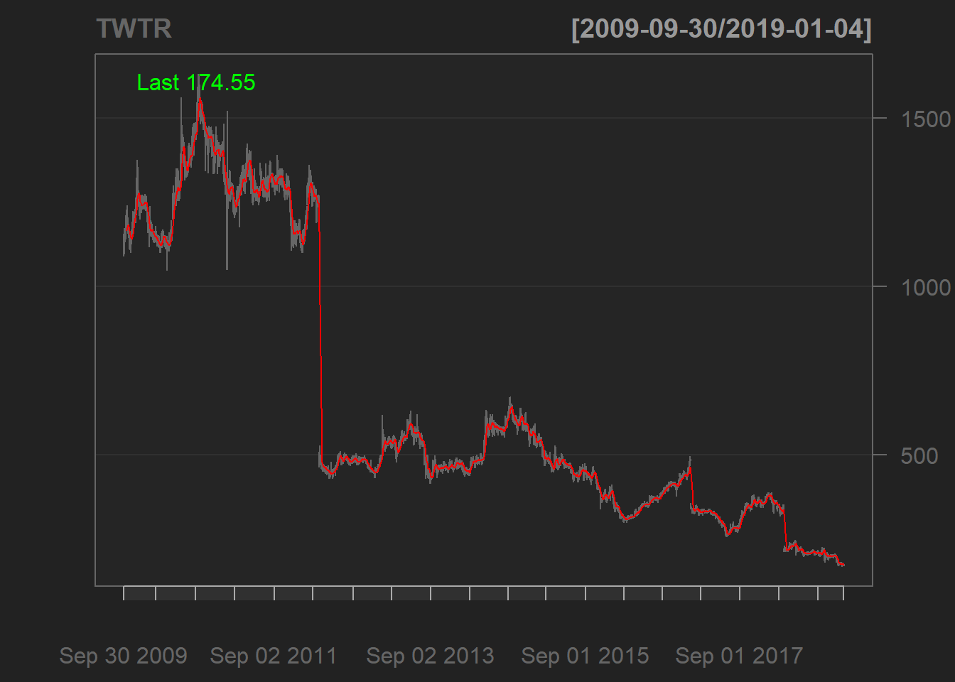
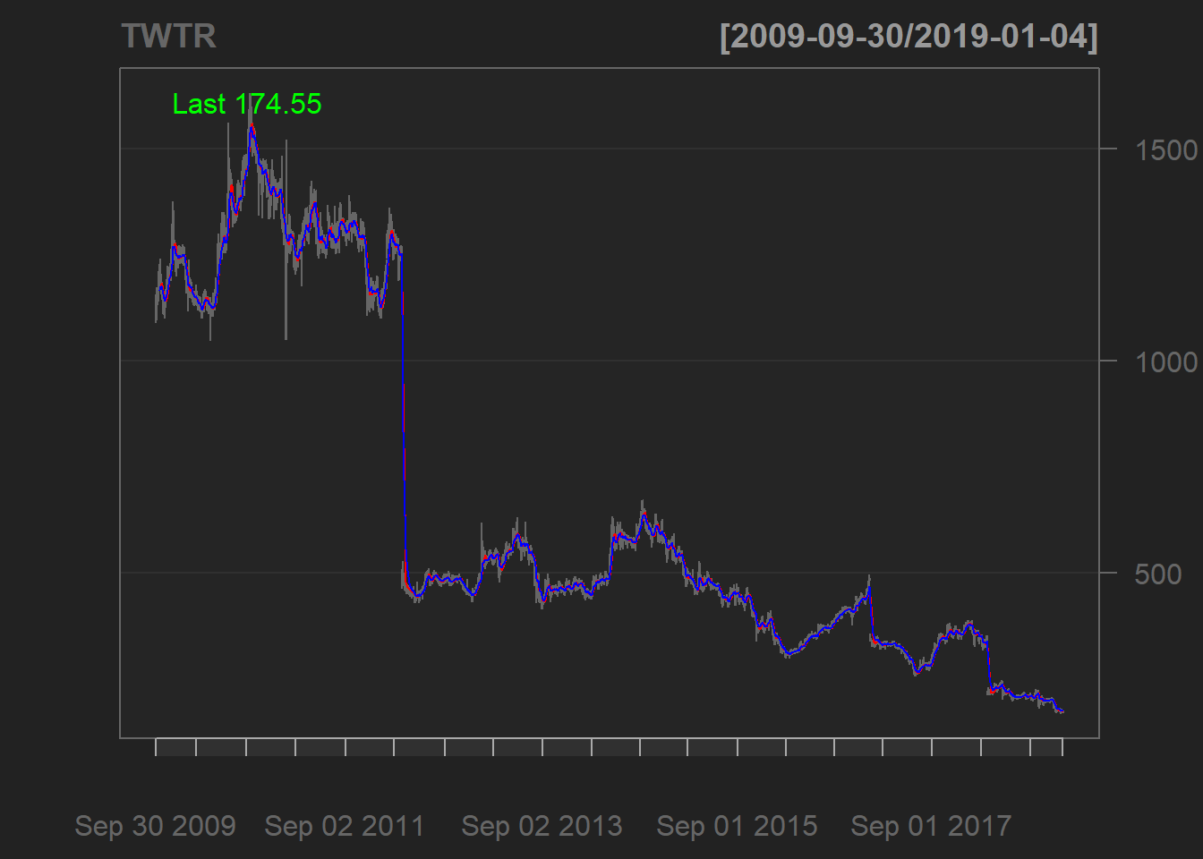
library("Quandl")
library("quantmod")
Quandl.auth("LDqWhYXzVd2omw4zipN2")
TWTR <- Quandl("NSE/OIL",type ="xts")
candleChart(TWTR)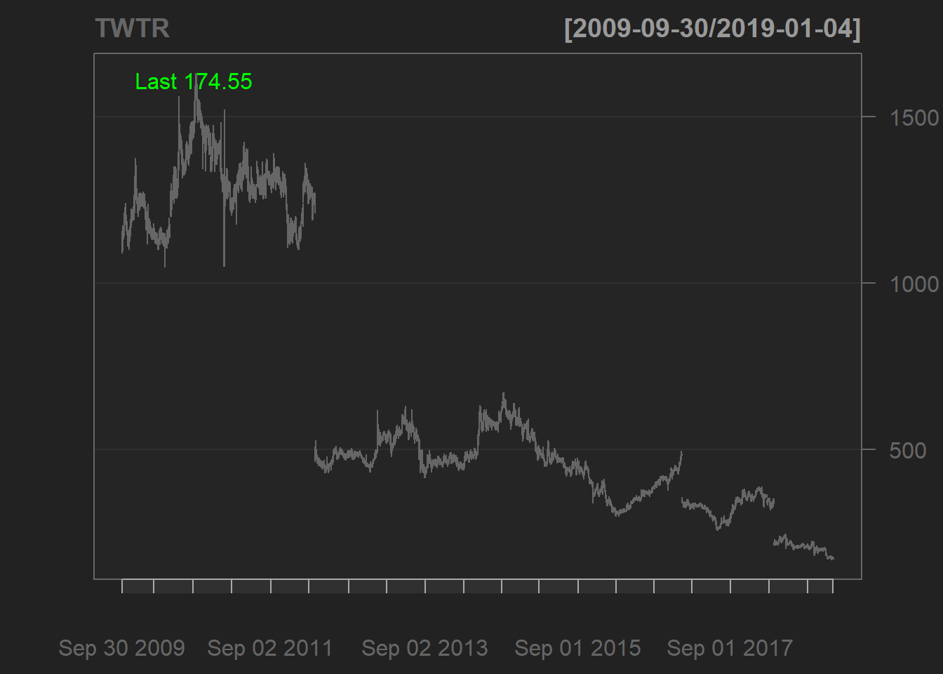
Reference market in Germany is DAX
# Index Data
# indexName <- c("DAX")

indexData <- tq_get("^GDAXI", from = "2014-05-01", to = "2015-12-31") %>%
    mutate(date = format(date, "%d.%m.%Y")) %>%
    mutate(symbol = "DAX")

head(indexData)
Create files
01_RequestFile.csv02_FirmData.csv03_MarketData.csv
Calculating abnormal returns
# get & set parameters for abnormal return Event Study
# we use a garch model and csv as return
# Attention: fitting a GARCH(1, 1) model is compute intensive
esaParams <- EventStudy::ARCApplicationInput$new()
esaParams$setResultFileType("csv")
esaParams$setBenchmarkModel("garch")


dataFiles <-
    c(
        "request_file" = file.path(getwd(), "data", "EventStudy", "01_requestFile.csv"),
        "firm_data"    = file.path(getwd(), "data", "EventStudy", "02_firmDataPrice.csv"),
        "market_data"  = file.path(getwd(), "data", "EventStudy", "03_marketDataPrice.csv")
    )

# check data files, you can do it also in our R6 class
EventStudy::checkFiles(dataFiles)
arEventStudy <- estSetup$performEventStudy(estParams = esaParams,
dataFiles = dataFiles,
downloadFiles = T)library(EventStudy)
apiUrl <- "https://api.eventstudytools.com"
Sys.setenv(EventStudyapiKey = "")
# The URL is already set by default
options(EventStudy.URL = apiUrl)
options(EventStudy.KEY = Sys.getenv("EventStudyapiKey"))
# use EventStudy estAPIKey function
estAPIKey(Sys.getenv("EventStudyapiKey"))
# initialize object
estSetup <- EventStudyAPI$new()
estSetup$authentication(apiKey = Sys.getenv("EventStudyapiKey"))