7.7 Generalization

We can see that Poisson regression looks similar to logistic regression. Hence, we can generalize to a class of modeling. Thanks to Nelder and Wedderburn (1972), we have the generalized linear models (GLMs). Estimation is generalize in these models.

Exponential Family
The theory of GLMs is developed for data with distribution given y the exponential family.
The form of the data distribution that is useful for GLMs is

\[ f(y;\theta, \phi) = \exp(\frac{\theta y - b(\theta)}{a(\phi)} + c(y, \phi)) \]

where

• \(\theta\) is called the natural parameter
• \(\phi\) is called the dispersion parameter

Note:

This family includes the Gamma, Normal, Poisson, and other. For all parameterization of the exponential family, check this link

Example

if we have \(Y \sim N(\mu, \sigma^2)\)

\[ \begin{aligned} f(y; \mu, \sigma^2) &= \frac{1}{(2\pi \sigma^2)^{1/2}}\exp(-\frac{1}{2\sigma^2}(y- \mu)^2) \\ &= \exp(-\frac{1}{2\sigma^2}(y^2 - 2y \mu +\mu^2)- \frac{1}{2}\log(2\pi \sigma^2)) \\ &= \exp(\frac{y \mu - \mu^2/2}{\sigma^2} - \frac{y^2}{2\sigma^2} - \frac{1}{2}\log(2\pi \sigma^2)) \\ &= \exp(\frac{\theta y - b(\theta)}{a(\phi)} + c(y , \phi)) \end{aligned} \]

where

• \(\theta = \mu\)
• \(b(\theta) = \frac{\mu^2}{2}\)
• \(a(\phi) = \sigma^2 = \phi\)
• \(c(y , \phi) = - \frac{1}{2}(\frac{y^2}{\phi}+\log(2\pi \sigma^2))\)

Properties of GLM exponential families

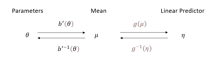
1. \(E(Y) = b' (\theta)\) where \(b'(\theta) = \frac{\partial b(\theta)}{\partial \theta}\) (here ' is “prime”, not transpose)

2. \(var(Y) = a(\phi)b''(\theta)= a(\phi)V(\mu)\).

   • \(V(\mu)\) is the variance function; however, it is only the variance in the case that \(a(\phi) =1\)

3. If \(a(), b(), c()\) are identifiable, we will derive expected value and variance of Y.

Example

Normal distribution

\[ \begin{aligned} b'(\theta) &= \frac{\partial b(\mu^2/2)}{\partial \mu} = \mu \\ V(\mu) &= \frac{\partial^2 (\mu^2/2)}{\partial \mu^2} = 1 \\ \to var(Y) &= a(\phi) = \sigma^2 \end{aligned} \]

Poisson distribution

\[ \begin{aligned} f(y, \theta, \phi) &= \frac{\mu^y \exp(-\mu)}{y!} \\ &= \exp(y\log(\mu) - \mu - \log(y!)) \\ &= \exp(y\theta - \exp(\theta) - \log(y!)) \end{aligned} \]

where

• \(\theta = \log(\mu)\)
• \(a(\phi) = 1\)
• \(b(\theta) = \exp(\theta)\)
• \(c(y, \phi) = \log(y!)\)

Hence,

\[ \begin{aligned} E(Y) = \frac{\partial b(\theta)}{\partial \theta} = \exp(\theta) &= \mu \\ var(Y) = \frac{\partial^2 b(\theta)}{\partial \theta^2} &= \mu \end{aligned} \]

Since \(\mu = E(Y) = b'(\theta)\)

In GLM, we take some monotone function (typically nonlinear) of \(\mu\) to be linear in the set of covariates

\[ g(\mu) = g(b'(\theta)) = \mathbf{x'\beta} \]

Equivalently,

\[ \mu = g^{-1}(\mathbf{x'\beta}) \]

where \(g(.)\) is the link function since it links mean response (\(\mu = E(Y)\)) and a linear expression of the covariates

Some people use \(\eta = \mathbf{x'\beta}\) where \(\eta\) = the “linear predictor”

GLM is composed of 2 components

The random component:

• is the distribution chosen to model the response variables \(Y_1,...,Y_n\)

• is specified by the choice fo \(a(), b(), c()\) in the exponential form

• Notation:

  • Assume that there are n independent response variables \(Y_1,...,Y_n\) with densities
    \[ f(y_i ; \theta_i, \phi) = \exp(\frac{\theta_i y_i - b(\theta_i)}{a(\phi)}+ c(y_i, \phi)) \] notice each observation might have different densities
  • Assume that \(\phi\) is constant for all \(i = 1,...,n\), but \(\theta_i\) will vary. \(\mu_i = E(Y_i)\) for all i.

The systematic component

• is the portion of the model that gives the relation between \(\mu\) and the covariates \(\mathbf{x}\)

• consists of 2 parts:

  • the link function, \(g(.)\)
  • the linear predictor, \(\eta = \mathbf{x'\beta}\)

• Notation:

  • assume \(g(\mu_i) = \mathbf{x'\beta} = \eta_i\) where \(\mathbf{\beta} = (\beta_1,..., \beta_p)'\)
  • The parameters to be estimated are \(\beta_1,...\beta_p , \phi\)

The Canonical Link

To choose \(g(.)\), we can use canonical link function (Remember: Canonical link is just a special case of the link function)

If the link function \(g(.)\) is such \(g(\mu_i) = \eta_i = \theta_i\), the natural parameter, then \(g(.)\) is the canonical link.

• \(b(\theta)\) = cumulant moment generating function
• \(g(\mu)\) is the link function, which relates the linear predictor to the mean and is required to be monotone increasing, continuously differentiable and invertible.

Equivalently, we can think of canonical link function as

\[ \gamma^{-1} \circ g^{-1} = I \] which is the identity. Hence,

\[ \theta = \eta \]

The inverse link

\(g^{-1}(.)\) is also known as the mean function, take linear predictor output (ranging from \(-\infty\) to \(\infty\)) and transform it into a different scale.

• Exponential: converts \(\mathbf{\beta X}\) into a curve that is restricted between 0 and \(\infty\) (which you can see that is useful in case you want to convert a linear predictor into a non-negative value). \(\lambda = \exp(y) = \mathbf{\beta X}\)

• Inverse Logit (also known as logistic): converts \(\mathbf{\beta X}\) into a curve that is restricted between 0 and 1, which is useful in case you want to convert a linear predictor to a probability. \(\theta = \frac{1}{1 + \exp(-y)} = \frac{1}{1 + \exp(- \mathbf{\beta X})}\)

  • \(y\) = linear predictor value
  • \(\theta\) = transformed value

The identity link is that

\[ \begin{aligned} \eta_i &= g(\mu_i) = \mu_i \\ \mu_i &= g^{-1}(\eta_i) = \eta_i \end{aligned} \]

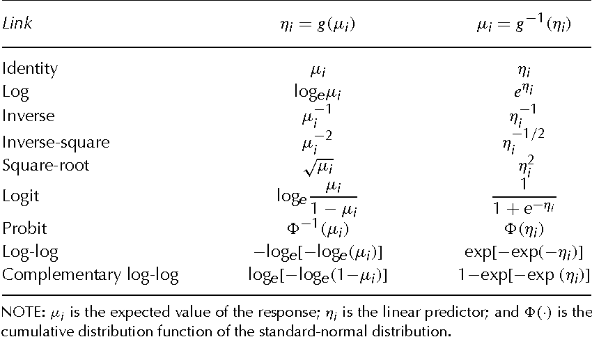
Table 15.1 Generalized Linear Models 15.1 the Structure of Generalized Linear Models

More example on the link functions and their inverses can be found on page 380

Example

Normal random component

• Mean Response: \(\mu_i = \theta_i\)

• Canonical Link: \(g( \mu_i) = \mu_i\) (the identity link)

Binomial random component

• Mean Response: \(\mu_i = \frac{n_i \exp( \theta)}{1+\exp (\theta_i)}\) and \(\theta(\mu_i) = \log(\frac{p_i }{1-p_i}) = \log (\frac{\mu_i} {n_i - \mu_i})\)

• Canonical link: \(g(\mu_i) = \log(\frac{\mu_i} {n_i - \mu_i})\) (logit link)

Poisson random component

• Mean Response: \(\mu_i = \exp(\theta_i)\)

• Canonical Link: \(g(\mu_i) = \log(\mu_i)\)

Gamma random component:

• Mean response: \(\mu_i = -\frac{1}{\theta_i}\) and \(\theta(\mu_i) = - \mu_i^{-1}\)

• Canonical Link: \(g(\mu\_i) = - \frac{1}{\mu_i}\)

Inverse Gaussian random

• Canonical Link: \(g(\mu_i) = \frac{1}{\mu_i^2}\)

7.7.1 Estimation

• MLE for parameters of the systematic component (\(\beta\))
• Unification of derivation and computation (thanks to the exponential forms)
• No unification for estimation of the dispersion parameter (\(\phi\))

7.7.1.1 Estimation of \(\beta\)

We have

\[ \begin{aligned} f(y_i ; \theta_i, \phi) &= \exp(\frac{\theta_i y_i - b(\theta_i)}{a(\phi)}+ c(y_i, \phi)) \\ E(Y_i) &= \mu_i = b'(\theta) \\ var(Y_i) &= b''(\theta)a(\phi) = V(\mu_i)a(\phi) \\ g(\mu_i) &= \mathbf{x}_i'\beta = \eta_i \end{aligned} \]

If the log-likelihood for a single observation is \(l_i (\beta,\phi)\). The log-likelihood for all n observations is

\[ \begin{aligned} l(\beta,\phi) &= \sum_{i=1}^n l_i (\beta,\phi) \\ &= \sum_{i=1}^n (\frac{\theta_i y_i - b(\theta_i)}{a(\phi)}+ c(y_i, \phi)) \end{aligned} \]

Using MLE to find \(\beta\), we use the chain rule to get the derivatives

\[ \begin{aligned} \frac{\partial l_i (\beta,\phi)}{\partial \beta_j} &= \frac{\partial l_i (\beta, \phi)}{\partial \theta_i} \times \frac{\partial \theta_i}{\partial \mu_i} \times \frac{\partial \mu_i}{\partial \eta_i}\times \frac{\partial \eta_i}{\partial \beta_j} \\ &= \sum_{i=1}^{n}(\frac{ y_i - \mu_i}{a(\phi)} \times \frac{1}{V(\mu_i)} \times \frac{\partial \mu_i}{\partial \eta_i} \times x_{ij}) \end{aligned} \]

If we let

\[ w_i \equiv ((\frac{\partial \eta_i}{\partial \mu_i})^2 V(\mu_i))^{-1} \]

Then,

\[ \frac{\partial l_i (\beta,\phi)}{\partial \beta_j} = \sum_{i=1}^n (\frac{y_i \mu_i}{a(\phi)} \times w_i \times \frac{\partial \eta_i}{\partial \mu_i} \times x_{ij}) \]

We can also get the second derivatives using the chain rule.

Example:

For the \[Newton-Raphson\] algorithm, we need

\[ - E(\frac{\partial^2 l(\beta,\phi)}{\partial \beta_j \partial \beta_k}) \]

where \((j,k)\)-th element of the Fisher information matrix \(\mathbf{I}(\beta)\)

Hence,

\[ - E(\frac{\partial^2 l(\beta,\phi)}{\partial \beta_j \partial \beta_k}) = \sum_{i=1}^n \frac{w_i}{a(\phi)}x_{ij}x_{ik} \]

for the (j,k)th element

If Bernoulli model with logit link function (which is the canonical link)

\[ \begin{aligned} b(\theta) &= \log(1 + \exp(\theta)) = \log(1 + \exp(\mathbf{x'\beta})) \\ a(\phi) &= 1 \\ c(y_i, \phi) &= 0 \\ E(Y) = b'(\theta) &= \frac{\exp(\theta)}{1 + \exp(\theta)} = \mu = p \\ \eta = g(\mu) &= \log(\frac{\mu}{1-\mu}) = \theta = \log(\frac{p}{1-p}) = \mathbf{x'\beta} \end{aligned} \]

For \(Y_i\), i = 1,.., the log-likelihood is

\[ l_i (\beta, \phi) = \frac{y_i \theta_i - b(\theta_i)}{a(\phi)} + c(y_i, \phi) = y_i \mathbf{x}'_i \beta - \log(1+ \exp(\mathbf{x'\beta})) \]

Additionally,

\[ \begin{aligned} V(\mu_i) &= \mu_i(1-\mu_i)= p_i (1-p_i) \\ \frac{\partial \mu_i}{\partial \eta_i} &= p_i(1-p_i) \end{aligned} \]

Hence,

\[ \begin{aligned} \frac{\partial l(\beta, \phi)}{\partial \beta_j} &= \sum_{i=1}^n[\frac{y_i - \mu_i}{a(\phi)} \times \frac{1}{V(\mu_i)}\times \frac{\partial \mu_i}{\partial \eta_i} \times x_{ij}] \\ &= \sum_{i=1}^n (y_i - p_i) \times \frac{1}{p_i(1-p_i)} \times p_i(1-p_i) \times x_{ij} \\ &= \sum_{i=1}^n (y_i - p_i) x_{ij} \\ &= \sum_{i=1}^n (y_i - \frac{\exp(\mathbf{x'_i\beta})}{1+ \exp(\mathbf{x'_i\beta})})x_{ij} \end{aligned} \]

then

\[ w_i = ((\frac{\partial \eta_i}{\partial \mu_i})^2 V(\mu_i))^{-1} = p_i (1-p_i) \]

\[ \mathbf{I}_{jk}(\mathbf{\beta}) = \sum_{i=1}^n \frac{w_i}{a(\phi)} x_{ij}x_{ik} = \sum_{i=1}^n p_i (1-p_i)x_{ij}x_{ik} \]

The Fisher-scoring algorithm for the MLE of \(\mathbf{\beta}\) is

\[ \left( \begin{array} {c} \beta_1 \\ \beta_2 \\ . \\ . \\ . \\ \beta_p \\ \end{array} \right)^{(m+1)} = \left( \begin{array} {c} \beta_1 \\ \beta_2 \\ . \\ . \\ . \\ \beta_p \\ \end{array} \right)^{(m)} + \mathbf{I}^{-1}(\mathbf{\beta}) \left( \begin{array} {c} \frac{\partial l (\beta, \phi)}{\partial \beta_1} \\ \frac{\partial l (\beta, \phi)}{\partial \beta_2} \\ . \\ . \\ . \\ \frac{\partial l (\beta, \phi)}{\partial \beta_p} \\ \end{array} \right)|_{\beta = \beta^{(m)}} \]

Similar to \[Newton-Raphson\] expect the matrix of second derivatives by the expected value of the second derivative matrix.

In matrix notation,

\[ \begin{aligned} \frac{\partial l }{\partial \beta} &= \frac{1}{a(\phi)}\mathbf{X'W\Delta(y - \mu)} \\ &= \frac{1}{a(\phi)}\mathbf{F'V^{-1}(y - \mu)} \\ \end{aligned} \]

\[ \mathbf{I}(\beta) = \frac{1}{a(\phi)}\mathbf{X'WX} = \frac{1}{a(\phi)}\mathbf{F'V^{-1}F} \]

where

• \(\mathbf{X}\) is an \(n \times p\) matrix of covariates
• \(\mathbf{W}\) is an \(n \times n\) diagonal matrix with \((i,i)\)-th element given by \(w_i\)
• \(\mathbf{\Delta}\) an \(n \times n\) diagonal matrix with \((i,i)\)-th element given by \(\frac{\partial \eta_i}{\partial \mu_i}\)
• \(\mathbf{F} = \mathbf{\frac{\partial \mu}{\partial \beta}}\) an \(n \times p\) matrix with \(i\)-th row \(\frac{\partial \mu_i}{\partial \beta} = (\frac{\partial \mu_i}{\partial \eta_i})\mathbf{x}'_i\)
• \(\mathbf{V}\) an \(n \times n\) diagonal matrix with \((i,i)\)-th element given by \(V(\mu_i)\)

Setting the derivative of the log-likelihood equal to 0, ML estimating equations are

\[ \mathbf{F'V^{-1}y= F'V^{-1}\mu} \]

where all components of this equation expect y depends on the parameters \(\beta\)

Special Cases

If one has a canonical link, the estimating equations reduce to

\[ \mathbf{X'y= X'\mu} \]

If one has an identity link, then

\[ \mathbf{X'V^{-1}y = X'V^{-1}X\hat{\beta}} \]

which gives the generalized least squares estimator

Generally, we can rewrite the Fisher-scoring algorithm as

\[ \beta^{(m+1)} = \beta^{(m)} + \mathbf{(\hat{F}'\hat{V}^{-1}\hat{F})^{-1}\hat{F}'\hat{V}^{-1}(y- \hat{\mu})} \]

Since \(\hat{F},\hat{V}, \hat{\mu}\) depend on \(\beta\), we evaluate at \(\beta^{(m)}\)

From starting values \(\beta^{(0)}\), we can iterate until convergence.

Notes:

• if \(a(\phi)\) is a constant or of the form \(m_i \phi\) with known \(m_i\), then \(\phi\) cancels.

7.7.1.2 Estimation of \(\phi\)

2 approaches:

1. MLE

\[ \frac{\partial l_i}{\partial \phi} = \frac{(\theta_i y_i - b(\theta_i)a'(\phi))}{a^2(\phi)} + \frac{\partial c(y_i,\phi)}{\partial \phi} \]

the MLE of \(\phi\) solves

\[ \frac{a^2(\phi)}{a'(\phi)}\sum_{i=1}^n \frac{\partial c(y_i, \phi)}{\partial \phi} = \sum_{i=1}^n(\theta_i y_i - b(\theta_i)) \]

• Situation others than normal error case, expression for \(\frac{\partial c(y,\phi)}{\partial \phi}\) are not simple

• Even for the canonical link and \(a(\phi)\) constant, there is no nice general expression for \(-E(\frac{\partial^2 l}{\partial \phi^2})\), so the unification GLMs provide for estimation of \(\beta\) breaks down for \(\phi\)

2. Moment Estimation (“Bias Corrected \(\chi^2\)”)

   • The MLE is not conventional approach to estimation of \(\phi\) in GLMS.
   • For the exponential family \(var(Y) =V(\mu)a(\phi)\). This implies
     \[ \begin{aligned} a(\phi) &= \frac{var(Y)}{V(\mu)} = \frac{E(Y- \mu)^2}{V(\mu)} \\ a(\hat{\phi}) &= \frac{1}{n-p} \sum_{i=1}^n \frac{(y_i -\hat{\mu}_i)^2}{V(\hat{\mu})} \end{aligned} \] where \(p\) is the dimension of \(\beta\)
   • GLM with canonical link function \(g(.)= (b'(.))^{-1}\)
     \[ \begin{aligned} g(\mu) &= \theta = \eta = \mathbf{x'\beta} \\ \mu &= g^{-1}(\eta)= b'(\eta) \end{aligned} \]
   • so the method estimator for \(a(\phi)=\phi\) is

\[ \hat{\phi} = \frac{1}{n-p} \sum_{i=1}^n \frac{(y_i - g^{-1}(\hat{\eta}_i))^2}{V(g^{-1}(\hat{\eta}_i))} \]

7.7.2 Inference

We have

\[ \hat{var}(\beta) = a(\phi)(\mathbf{\hat{F}'\hat{V}\hat{F}})^{-1} \]

where

• \(\mathbf{V}\) is an \(n \times n\) diagonal matrix with diagonal elements given by \(V(\mu_i)\)
• \(\mathbf{F}\) is an \(n \times p\) matrix given by \(\mathbf{F} = \frac{\partial \mu}{\partial \beta}\)
• Both \(\mathbf{V,F}\) are dependent on the mean \(\mu\), and thus \(\beta\). Hence, their estimates (\(\mathbf{\hat{V},\hat{F}}\)) depend on \(\hat{\beta}\).

\[ H_0: \mathbf{L\beta = d} \]

where \(\mathbf{L}\) is a q x p matrix with a Wald test

\[ W = \mathbf{(L \hat{\beta}-d)'(a(\phi)L(\hat{F}'\hat{V}^{-1}\hat{F})L')^{-1}(L \hat{\beta}-d)} \]

which follows \(\chi_q^2\) distribution (asymptotically), where \(q\) is the rank of \(\mathbf{L}\)

In the simple case \(H_0: \beta_j = 0\) gives \(W = \frac{\hat{\beta}^2_j}{\hat{var}(\hat{\beta}_j)} \sim \chi^2_1\) asymptotically

Likelihood ratio test

\[ \Lambda = 2 (l(\hat{\beta}_f)-l(\hat{\beta}_r)) \sim \chi^2_q \]

where

• \(q\) is the number of constraints used to fit the reduced model \(\hat{\beta}_r\), and \(\hat{\beta}_r\) is the fit under the full model.

Wald test is easier to implement, but likelihood ratio test is better (especially for small samples).

7.7.3 Deviance

Deviance is necessary for goodness of fit, inference and for alternative estimation of the dispersion parameter. We define and consider Deviance from a likelihood ratio perspective.

• Assume that \(\phi\) is known. Let \(\tilde{\theta}\) denote the full and \(\hat{\theta}\) denote the reduced model MLEs. Then, the likelihood ratio (2 times the difference in log-likelihoods) is \[ 2\sum_{i=1}^{n} \frac{y_i (\tilde{\theta}_i- \hat{\theta}_i)-b(\tilde{\theta}_i) + b(\hat{\theta}_i)}{a_i(\phi)} \]

• For exponential families, \(\mu = E(y) = b'(\theta)\), so the natural parameter is a function of \(\mu: \theta = \theta(\mu) = b'^{-1}(\mu)\), and the likelihood ratio turns into
  \[ 2 \sum_{i=1}^m \frac{y_i\{\theta(\tilde{\mu}_i - \theta(\hat{\mu}_i)\} - b(\theta(\tilde{\mu}_i)) + b(\theta(\hat{\mu}_i))}{a_i(\phi)} \]

• Comparing a fitted model to “the fullest possible model”, which is the saturated model: \(\tilde{\mu}_i = y_i\), i = 1,..,n. If \(\tilde{\theta}_i^* = \theta(y_i), \hat{\theta}_i^* = \theta (\hat{\mu})\), the likelihood ratio is
  \[ 2 \sum_{i=1}^{n} \frac{y_i (\tilde{\theta}_i^* - \hat{\theta}_i^* + b(\hat{\theta}_i^*))}{a_i(\phi)} \]

• (McCullagh 2019) specify \(a(\phi) = \phi\), then the likelihood ratio can be written as
  \[ D^*(\mathbf{y, \hat{\mu}}) = \frac{2}{\phi}\sum_{i=1}^n\{y_i (\tilde{\theta}_i^*- \hat{\theta}_i^*)- b(\tilde{\theta}_i^*) +b(\hat{\theta}_i^*) \} \] where

• \(D^*(\mathbf{y, \hat{\mu}})\) = scaled deviance

• \(D(\mathbf{y, \hat{\mu}}) = \phi D^*(\mathbf{y, \hat{\mu}})\) = deviance

Note:

• in some random component distributions, we can write \(a_i(\phi) = \phi m_i\), where

  • \(m_i\) is some known scalar that may change with the observations. Then, the scaled deviance components are divided by \(m_i\):
    \[ D^*(\mathbf{y, \hat{\mu}}) \equiv 2\sum_{i=1}^n\{y_i (\tilde{\theta}_i^*- \hat{\theta}_i^*)- b(\tilde{\theta}_i^*) +b(\hat{\theta}_i^*)\} / (\phi m_i) \]

• \(D^*(\mathbf{y, \hat{\mu}}) = \sum_{i=1}^n d_i\)m where \(d_i\) is the deviance contribution from the \(i\)-th observation.

• \(D\) is used in model selection

• \(D^*\) is used in goodness of fit tests (as it is a likelihood ratio statistic). \[ D^*(\mathbf{y, \hat{\mu}}) = 2\{l(\mathbf{y,\tilde{\mu}})-l(\mathbf{y,\hat{\mu}})\} \]

• \(d_i\) are used to form deviance residuals

Normal

We have

\[ \begin{aligned} \theta &= \mu \\ \phi &= \sigma^2 \\ b(\theta) &= \frac{1}{2} \theta^2 \\ a(\phi) &= \phi \end{aligned} \]

Hence,

\[ \begin{aligned} \tilde{\theta}_i &= y_i \\ \hat{\theta}_i &= \hat{\mu}_i = g^{-1}(\hat{\eta}_i) \end{aligned} \]

And

\[ \begin{aligned} D &= 2 \sum_{1=1}^n Y^2_i - y_i \hat{\mu}_i - \frac{1}{2}y^2_i + \frac{1}{2} \hat{\mu}_i^2 \\ &= \sum_{i=1}^n y_i^2 - 2y_i \hat{\mu}_i + \hat{\mu}_i^2 \\ &= \sum_{i=1}^n (y_i - \hat{\mu}_i)^2 \end{aligned} \]

which is the residual sum of squares

Poisson

\[ \begin{aligned} f(y) &= \exp\{y\log(\mu) - \mu - \log(y!)\} \\ \theta &= \log(\mu) \\ b(\theta) &= \exp(\theta) \\ a(\phi) &= 1 \\ \tilde{\theta}_i &= \log(y_i) \\ \hat{\theta}_i &= \log(\hat{\mu}_i) \\ \hat{\mu}_i &= g^{-1}(\hat{\eta}_i) \end{aligned} \]

Then,

\[ \begin{aligned} D &= 2 \sum_{i = 1}^n y_i \log(y_i) - y_i \log(\hat{\mu}_i) - y_i + \hat{\mu}_i \\ &= 2 \sum_{i = 1}^n y_i \log(\frac{y_i}{\hat{\mu}_i}) - (y_i - \hat{\mu}_i) \end{aligned} \]

and

\[ d_i = 2\{y_i \log(\frac{y_i}{\hat{\mu}})- (y_i - \hat{\mu}_i)\} \]

7.7.3.1 Analysis of Deviance

The difference in deviance between a reduced and full model, where q is the difference in the number of free parameters, has an asymptotic \(\chi^2_q\). The likelihood ratio test

\[ D^*(\mathbf{y;\hat{\mu}_r}) - D^*(\mathbf{y;\hat{\mu}_f}) = 2\{l(\mathbf{y;\hat{\mu}_f})-l(\mathbf{y;\hat{\mu}_r})\} \]

this comparison of models is Analysis of Deviance. GLM uses this analysis for model selection.

An estimation of \(\phi\) is

\[ \hat{\phi} = \frac{D(\mathbf{y, \hat{\mu}})}{n - p} \]

where \(p\) = number of parameters fit.

Excessive use of \(\chi^2\) test could be problematic since it is asymptotic (McCullagh 2019)

7.7.3.2 Deviance Residuals

We have \(D = \sum_{i=1}^{n}d_i\). Then, we define deviance residuals

\[ r_{D_i} = \text{sign}(y_i -\hat{\mu}_i)\sqrt{d_i} \]

Standardized version of deviance residuals is

\[ r_{s,i} = \frac{y_i -\hat{\mu}}{\hat{\sigma}(1-h_{ii})^{1/2}} \]

Let \(\mathbf{H^{GLM} = W^{1/2}X(X'WX)^{-1}X'W^{-1/2}}\), where \(\mathbf{W}\) is an \(n \times n\) diagonal matrix with \((i,i)\)-th element given by \(w_i\) (see Estimation of \(\beta\)). Then Standardized deviance residuals is equivalently

\[ r_{s, D_i} = \frac{r_{D_i}}{\{\hat{\phi}(1-h_{ii}^{glm}\}^{1/2}} \]

where \(h_{ii}^{glm}\) is the \(i\)-th diagonal of \(\mathbf{H}^{GLM}\)

7.7.3.3 Pearson Chi-square Residuals

Another \(\chi^2\) statistic is Pearson \(\chi^2\) statistics: (assume \(m_i = 1\))

\[ X^2 = \sum_{i=1}^{n} \frac{(y_i - \hat{\mu}_i)^2}{V(\hat{\mu}_i)} \]

where \(\hat{\mu}_i\) is the fitted mean response fo the model of interest.

The Scaled Pearson \(\chi^2\) statistic is given by \(\frac{X^2}{\phi} \sim \chi^2_{n-p}\) where p is the number of parameters estimated. Hence, the Pearson \(\chi^2\) residuals are

\[ X^2_i = \frac{(y_i - \hat{\mu}_i)^2}{V(\hat{\mu}_i)} \]

If we have the following assumptions:

• Independent samples
  
• No over-dispersion: If \(\phi = 1\), \(\frac{D(\mathbf{y;\hat{\mu}})}{n-p}\) and \(\frac{X^2}{n-p}\) have a value substantially larger 1 indicates improperly specified model or overdispersion
  
• Multiple groups

then \(\frac{X^2}{\phi}\) and \(D^*(\mathbf{y; \hat{\mu}})\) both follow \(\chi^2_{n-p}\)

7.7.4 Diagnostic Plots

• Standardized residual Plots:

  • plot(\(r_{s, D_i}\), \(\hat{\mu}_i\)) or plot(\(r_{s, D_i}\), \(T(\hat{\mu}_i)\)) where \(T(\hat{\mu}_i)\) is transformation(\(\hat{\mu}_i\)) called constant information scale:
    
  • plot(\(r_{s, D_i}\), \(\hat{\eta}_i\))

Random Component	\(T(\hat{\mu}_i)\)
Normal	\(\hat{\mu}\)
Poisson	\(2\sqrt{\mu}\)
Binomial	\(2 \sin^{-1}(\sqrt{\hat{\mu}})\)
Gamma	\(2 \log(\hat{\mu})\)
Inverse Gaussian	\(-2\hat{\mu}^{-1/2}\)

• If we see:

  • Trend, it means we might have a wrong link function, or choice of scale
    
  • Systematic change in range of residuals with a change in \(T(\hat{\mu})\) (incorrect random component) (systematic \(\neq\) random)

• plot(\(|r_{D_i}|,\hat{\mu}_i\)) to check Variance Function.

7.7.5 Goodness of Fit

To assess goodness of fit, we can use

• Deviance
• Pearson Chi-square Residuals

In nested model, we could use likelihood-based information measures:

\[ \begin{aligned} AIC &= -2l(\mathbf{\hat{\mu}}) + 2p \\ AICC &= -2l(\mathbf{\hat{\mu}}) + 2p(\frac{n}{n-p-1}) \\ BIC &= 2l(\hat{\mu}) + p \log(n) \end{aligned} \]

where

• \(l(\hat{\mu})\) is the log-likelihood evaluated at the parameter estimates
• \(p\) is the number of parameters
• \(n\) is the number of observations.

Note: you have to use the same data with the same model (i.e., same link function, same random underlying random distribution). but you can have different number of parameters.

Even though statisticians try to come up with measures that are similar to \(R^2\), in practice, it is not so appropriate. For example, they compare the log-likelihood of the fitted model against the that of a model with just the intercept:

\[ R^2_p = 1 - \frac{l(\hat{\mu})}{l(\hat{\mu}_0)} \]

For certain specific random components such as binary response model, we have rescaled generalized \(R^2\)

\[ \bar{R}^2 = \frac{R^2_*}{\max(R^2_*)} = \frac{1-\exp\{-\frac{2}{n}(l(\hat{\mu}) - l(\hat{\mu}_0) \}}{1 - \exp\{\frac{2}{n}l(\hat{\mu}_0)\}} \]

7.7.6 Over-Dispersion

Random Components	\(var(Y)\)	\(V(\mu)\)
Binomial	\(var(Y) = n \mu (1- \mu)\)	\(V(\mu) = \phi n \mu(1- \mu)\) where \(m_i =n\)
Poisson	\(var(Y) = \mu\)	\(V(\mu) = \phi \mu\)

In both cases \(\phi = 1\). Recall \(b''(\theta)= V(\mu)\) check Estimation of \(\phi\).

If we find

• \(\phi >1\): over-dispersion (i.e., too much variation for an independent binomial or Poisson distribution).
• \(\phi<1\): under-dispersion (i.e., too little variation for an independent binomial or Poisson distribution).

If we have either over or under-dispersion, it means we might have unspecified random component, we could

• Select a different random component distribution that can accommodate over or under-dispersion (e.g., negative binomial, Conway-Maxwell Poisson)
• use Nonlinear and Generalized Linear Mixed Models to handle random effects in generalized linear models.

References

McCullagh, Peter. 2019. Generalized Linear Models. Routledge.

Nelder, John Ashworth, and Robert WM Wedderburn. 1972. “Generalized Linear Models.” Journal of the Royal Statistical Society Series A: Statistics in Society 135 (3): 370–84.