25 Synthetic Difference-in-Differences
also known as weighted double-differencing estimators
-
Setting: Researchers use panel data to study effects of policy changes.
Panel data: repeated observations across time for various units.
Some units exposed to policy at different times than others.
-
Policy changes often aren’t random across units or time.
- Challenge: Observed covariates might not lead to credible conclusions of no confounding (G. W. Imbens and Rubin 2015)
-
To estimate the effects, either
Difference-in-differences (DID) method widely used in applied economics.
Synthetic Control (SC) methods offer alternative approach for comparative case studies.
-
Difference between DID and SC:
DID: used with many policy-exposed units; relies on “parallel trends” assumption.
SC: used with few policy-exposed units; compensates lack of parallel trends by reweighting units based on pre-exposure trends.
-
New proposition: Synthetic Difference in Differences (SDID).
Combines features of DID and SC.
Reweights and matches pre-exposure trends (similar to SC).
Invariant to additive unit-level shifts, valid for large-panel inference (like DID).
-
Attractive features:
SDID provides consistent and asymptotically normal estimates.
-
SDID performs on par with or better than DID in traditional DID settings.
- where DID can only handle completely random treatment assignment, SDID can handle cases where treatment assignment is correlated with some time or unit latent factors.
Similarly, SDID is as good as or better than SC in traditional SC settings.
Uniformly random treatment assignment results in unbiased outcomes for all methods, but SDID is more precise.
SDID reduces bias effectively for non-uniformly random assignments.
SDID’s double robustness is akin to the augmented inverse probability weighting estimator Scharfstein, Rotnitzky, and Robins (1999).
Very much similar to augmented SC estimator by (Ben-Michael, Feller, and Rothstein 2021; Arkhangelsky et al. 2021, 4112)
Ideal case to use SDID estimator is when
\(N_{ctr} \approx T_{pre}\)
Small \(T_{post}\)
\(N_{tr} <\sqrt{N_{ctr}}\)
Applications in marketing:
Lambrecht, Tucker, and Zhang (2024): TV ads on online browsing and sales.
Keller, Guyt, and Grewal (2024): soda tax on marketing effectiveness.
25.1 Understanding
Consider a traditional time-series cross-sectional data
Let \(Y_{it}\) denote the outcome for unit \(i\) in period \(t\)
A balanced panel of \(N\) units and \(T\) time periods
\(W_{it} \in \{0, 1\}\) is the binary treatment
\(N_c\) never-treated units (control)
\(N_t\) treated units after time \(T_{pre}\)
Steps:
- Find unit weights \(\hat{w}^{sdid}\) such that \(\sum_{i = 1}^{N_c} \hat{w}_i^{sdid} Y_{it} \approx N_t^{-1} \sum_{i = N_c + 1}^N Y_{it} \forall t = 1, \dots, T_{pre}\) (i.e., pre-treatment trends in outcome of the treated similar to those of control units) (similar to SC).
- Find time weights \(\hat{\lambda}_t\) such that we have a balanced window (i.e., posttreatment outcomes for control units differ consistently from their weighted average pretreatment outcomes).
- Estimate the average causal effect of treatment
\[ (\hat{\tau}^{sdid}, \hat{\mu}, \hat{\alpha}, \hat{\beta}) = \arg \min_{\tau, \mu, \alpha, \beta} \{ \sum_{i = 1}^N \sum_{t = 1}^T (Y_{it} - \mu - \alpha_i - \beta_ t - W_{it} \tau)^2 \hat{w}_i^{sdid} \hat{\lambda}_t^{sdid} \} \]
Better than DiD estimator because \(\tau^{did}\) does not consider time or unit weights
\[ (\hat{\tau}^{did}, \hat{\mu}, \hat{\alpha}, \hat{\beta}) = \arg \min_{\tau, \mu, \alpha, \beta} \{ \sum_{i = 1}^N \sum_{t = 1}^T (Y_{it} - \mu - \alpha_i - \beta_ t - W_{it} \tau)^2 \} \]
Better than SC estimator because \(\tau^{sc}\) lacks unit fixed effete and time weights
\[ (\hat{\tau}^{sc}, \hat{\mu}, \hat{\beta}) = \arg \min_{\tau, \mu, \beta} \{ \sum_{i = 1}^N \sum_{t = 1}^T (Y_{it} - \mu - \beta_ t - W_{it} \tau)^2 \hat{w}_i^{sdid} \} \]
| DID | SC | SDID | |
|---|---|---|---|
| Primary Assumption | Absence of intervention leads to parallel evolution across states. | Reweights unexposed states to match pre-intervention outcomes of treated state. | Reweights control units to ensure a parallel time trend with the treated pre-intervention trend. |
| Reliability Concern | Can be unreliable when pre-intervention trends aren’t parallel. | Accounts for non-parallel pre-intervention trends by reweighting. | Uses reweighting to adjust for non-parallel pre-intervention trends. |
| Treatment of Time Periods | All pre-treatment periods are given equal weight. | Doesn’t specifically emphasize equal weight for pre-treatment periods. | Focuses only on a subset of pre-intervention time periods, selected based on historical outcomes. |
| Goal with Reweighting | N/A (doesn’t use reweighting). | To match treated state as closely as possible before the intervention. | Make trends of control units parallel (not necessarily identical) to the treated pre-intervention. |
Alternatively, think of our parameter of interest as:
\[ \hat{\tau} = \hat{\delta}_t - \sum_{i = 1}^{N_c} \hat{w}_i \hat{\delta}_i \]
where \(\hat{\delta}_t = \frac{1}{N_t} \sum_{i = N_c + 1}^N \hat{\delta}_i\)
| Method | Sample Weight | Adjusted outcomes (\(\hat{\delta}_i\)) | Interpretation |
|---|---|---|---|
| SC | \(\hat{w}^{sc} = \min_{w \in R}l_{unit}(w)\) | \(\frac{1}{T_{post}} \sum_{t = T_{pre} + 1}^T Y_{it}\) | Unweighted treatment period averages |
| DID | \(\hat{w}_i^{did} = N_c^{-1}\) | \(\frac{1}{T_{post}} \sum_{t = T_{pre}+ 1}^T Y_{it} - \frac{1}{T_{pre}} \sum_{t = 1}^{T_{pre}}Y_{it}\) | Unweighted differences between average treatment period and pretreatment outcome |
| SDID | \((\hat{w}_0, \hat{w}^{sdid}) = \min l_{unit}(w_0, w)\) | \(\frac{1}{T_{post}} \sum_{t = T_{pre} + 1}^T Y_{it} - \sum_{t = 1}^{T_{pre}} \hat{\lambda}_t^{sdid} Y_{it}\) | Weighted differences between average treatment period and pretreatment outcome |
-
The SDID estimator uses weights:
Makes two-way fixed effect regression “local.”
Emphasizes units similar in their past to treated units.
Prioritizes periods resembling treated periods.
-
Benefits of this localization:
Robustness: Using similar units and periods boosts estimator’s robustness.
-
Improved Precision: Weights can eliminate predictable outcome components.
The SEs of SDID are smaller than those of SC and DID
Caveat: If there’s minor systematic heterogeneity in outcomes, unequal weighting might reduce precision compared to standard DID.
-
Weight Design:
Unit Weights: Makes average outcome for treated units roughly parallel to the weighted average for control units.
Time Weights: Ensures posttreatment outcomes for control units differ consistently from their weighted average pretreatment outcomes.
-
Weights enhance DID’s plausibility:
Raw data often lacks parallel time trends for treated/control units.
Similar techniques (e.g., adjusting for covariates or selecting specific time periods) were used before (Callaway and Sant’Anna 2021).
SDID automates this process, applying a similar logic to weight both units and time periods.
-
Time Weights in SDID:
- Removes bias and boosts precision (i.e., minimizes the influence of time periods vastly different from posttreatment periods).
-
Argument for Unit Fixed Effects:
Flexibility: Increases model flexibility and thereby bolsters robustness.
Enhanced Precision: Unit fixed effects explain a significant portion of outcome variation.
-
SC Weighting & Unit Fixed Effects:
-
Under certain conditions, SC weighting can inherently account for unit fixed effects.
- For example, when the weighted average outcome for control units in pretreatment is the same as that of the treated units. (unlikely in reality)
The use of unit fixed effect in synthetic control regression (i.e., synthetic control with intercept) was proposed before in Doudchenko and Imbens (2016) and Ferman and Pinto (2021) (called DIFP)
-
More details on application
- Choose unit weights
-
Regularization Parameter:
- Equal to the size of a typical one-period outcome change for control units in the pre-period, then multiplied by a scaling factor (Arkhangelsky et al. 2021, 4092).
-
Relation to SC Weights:
-
SDID weights are similar to those used in (Abadie, Diamond, and Hainmueller 2010) except two distinctions:
-
Inclusion of an Intercept Term:
The weights in SynthDiD do not necessarily make the control pre-trends perfectly match the treated trends, just make them parallel.
This flexibility comes from the use of unit fixed effects, which can absorb any consistent differences between units.
-
Regularization Penalty:
Adopted from Doudchenko and Imbens (2016) .
Enhances the dispersion and ensures the uniqueness of the weights.
-
DID weights are identical to those used in (Abadie, Diamond, and Hainmueller 2010) without intercept and regularization penalty and 1 treated unit.
-
- Choose time weights
- Also include an intercept term, but no regularization (because correlated observations within time periods for the same unit is plausible, but not across units within the same period).
Note: To account for time-varying variables in the weights, one can use the residuals of the regression of the observed outcome on these time-varying variables, instead of the observed outcomes themselves (\(Y_{it}^{res} = Y_{it} - X_{it} \hat{\beta}\), where \(\hat{\beta}\) come from \(Y = \beta X_{it}\)).
The SDID method can account for systematic effects, often referred to as unit effects or unit heterogeneity, which influence treatment assignment (i.e., when treatment assignment is correlated with these systematic effects). Consequently, it provides unbiased estimates, especially valuable when there’s a suspicion that the treatment might be influenced by persistent, unit-specific attributes.
Even in cases where we have completely random assignment, SDID, DiD, and SC are unbiased, but SynthDiD has the smallest SE.
25.2 Application
SDID Algorithm
- Compute regularization parameter \(\zeta\)
\[ \zeta = (N_{t}T_{post})^{1/4} \hat{\sigma} \]
where
\[ \hat{\sigma}^2 = \frac{1}{N_c(T_{pre}- 1)} \sum_{i = 1}^{N_c} \sum_{t = 1}^{T_{re}-1}(\Delta_{it} - \hat{\Delta})^2 \]
\(\Delta_{it} = Y_{i(t + 1)} - Y_{it}\)
\(\hat{\Delta} = \frac{1}{N_c(T_{pre} - 1)}\sum_{i = 1}^{N_c}\sum_{t = 1}^{T_{pre}-1} \Delta_{it}\)
- Compute unit weights \(\hat{w}^{sdid}\)
\[ (\hat{w}_0, \hat{w}^{sidid}) = \arg \min_{w_0 \in R, w \in \Omega}l_{unit}(w_0, w) \]
where
\(l_{unit} (w_0, w) = \sum_{t = 1}^{T_{pre}}(w_0 + \sum_{i = 1}^{N_c}w_i Y_{it} - \frac{1}{N_t}\sum_{i = N_c + 1}^NY_{it})^2 + \zeta^2 T_{pre}||w||_2^2\)
\(\Omega = \{w \in R_+^N: \sum_{i = 1}^{N_c} w_i = 1, w_i = N_t^{-1} \forall i = N_c + 1, \dots, N \}\)
- Compute time weights \(\hat{\lambda}^{sdid}\)
\[ (\hat{\lambda}_0 , \hat{\lambda}^{sdid}) = \arg \min_{\lambda_0 \in R, \lambda \in \Lambda} l_{time}(\lambda_0, \lambda) \]
where
\(l_{time} (\lambda_0, \lambda) = \sum_{i = 1}^{N_c}(\lambda_0 + \sum_{t = 1}^{T_{pre}} \lambda_t Y_{it} - \frac{1}{T_{post}} \sum_{t = T_{pre} + 1}^T Y_{it})^2\)
\(\Lambda = \{ \lambda \in R_+^T: \sum_{t = 1}^{T_{pre}} \lambda_t = 1, \lambda_t = T_{post}^{-1} \forall t = T_{pre} + 1, \dots, T\}\)
- Compute the SDID estimator
\[ (\hat{\tau}^{sdid}, \hat{\mu}, \hat{\alpha}, \hat{\beta}) = \arg \min_{\tau, \mu, \alpha, \beta}\{ \sum_{i = 1}^N \sum_{t = 1}^T (Y_{it} - \mu - \alpha_i - \beta_t - W_{it} \tau)^2 \hat{w}_i^{sdid}\hat{\lambda}_t^{sdid} \]
SE Estimation
Under certain assumptions (errors, samples, and interaction properties between time and unit fixed effects) detailed in (Arkhangelsky et al. 2019, 4107), SDID is asymptotically normal and zero-centered
Using its asymptotic variance, conventional confidence intervals can be applied to SDID.
\[ \tau \in \hat{\tau}^{sdid} \pm z_{\alpha/2}\sqrt{\hat{V}_\tau} \]
-
There are 3 approaches for variance estimation in confidence intervals:
-
Clustered Bootstrap (Efron 1992):
Independently resample units.
Advantages: Simple to use; robust performance in large panels due to natural approach to inference with panel data where observations of the same unit might be correlated.
Disadvantage: Computationally expensive.
-
Jackknife (Miller 1974):
Applied to weighted SDID regression with fixed weights.
Generally conservative and precise when treated and control units are sufficiently similar.
Not recommended for some methods, like the SC estimator, due to potential biases.
Appropriate for jackknifing DID without random weights.
-
Placebo Variance Estimation:
Can used in cases with only one treated unit or large panels.
Placebo evaluations swap out the treated unit for untreated ones to estimate noise.
Relies on homoskedasticity across units.
Depends on homoskedasticity across units. It hinges on the empirical distribution of residuals from placebo estimators on control units.
The validity of the placebo method hinges on consistent noise distribution across units. One treated unit makes nonparametric variance estimation difficult, necessitating homoskedasticity for feasible inference. Detailed analysis available in Conley and Taber (2011).
-
All algorithms are from Arkhangelsky et al. (2021), p. 4109:
Bootstrap Variance Estimation
For each \(b\) from \(1 \to B\):
Sample \(N\) rows from \((\mathbf{Y}, \mathbf{W})\) to get (\(\mathbf{Y}^{(b)}, \mathbf{W}^{(b)}\)) with replacement.
If the sample lacks treated or control units, resample.
Calculate \(\tau^{(b)}\) using (\(\mathbf{Y}^{(b)}, \mathbf{W}^{(b)}\)).
Calculate variance: \(\hat{V}_\tau = \frac{1}{B} \sum_{b = 1}^B (\hat{\tau}^{b} - \frac{1}{B} \sum_{b = 1}^B \hat{\tau}^b)^2\)
Jackknife Variance Estimation
- For each \(i\) from \(1 \to N\):
- Calculate \(\hat{\tau}^{(-i)}\): \(\arg\min_{\tau, \{\alpha_j, \beta_t\}} \sum_{j \neq, i, t}(\mathbf{Y}_{jt} - \alpha_j - \beta_t - \tau \mathbf{W}_{it})^2 \hat{w}_j \hat{\lambda}_t\)
- Calculate: \(\hat{V}_{\tau} = (N - 1) N^{-1} \sum_{i = 1}^N (\hat{\tau}^{(-i)} - \hat{\tau})^2\)
Placebo Variance Estimation
- For each \(b\) from \(1 \to B\)
- Sample \(N_t\) out of \(N_c\) without replacement to get the “placebo” treatment
- Construct a placebo treatment matrix \(\mathbf{W}_c^b\) for the controls
- Calculate \(\hat{\tau}\) based on \((\mathbf{Y}_c, \mathbf{W}_c^b)\)
- Calculate \(\hat{V}_\tau = \frac{1}{B}\sum_{b = 1}^B (\hat{\tau}^b - \frac{1}{B} \sum_{b = 1}^B \hat{\tau}^b)^2\)
25.2.1 Block Treatment
Code provided by the synthdid package
library(synthdid)
library(tidyverse)

# Estimate the effect of California Proposition 99 on cigarette consumption
data('california_prop99')

setup = synthdid::panel.matrices(synthdid::california_prop99)

tau.hat = synthdid::synthdid_estimate(setup$Y, setup$N0, setup$T0)

# se = sqrt(vcov(tau.hat, method = 'placebo'))

plot(tau.hat) + causalverse::ama_theme()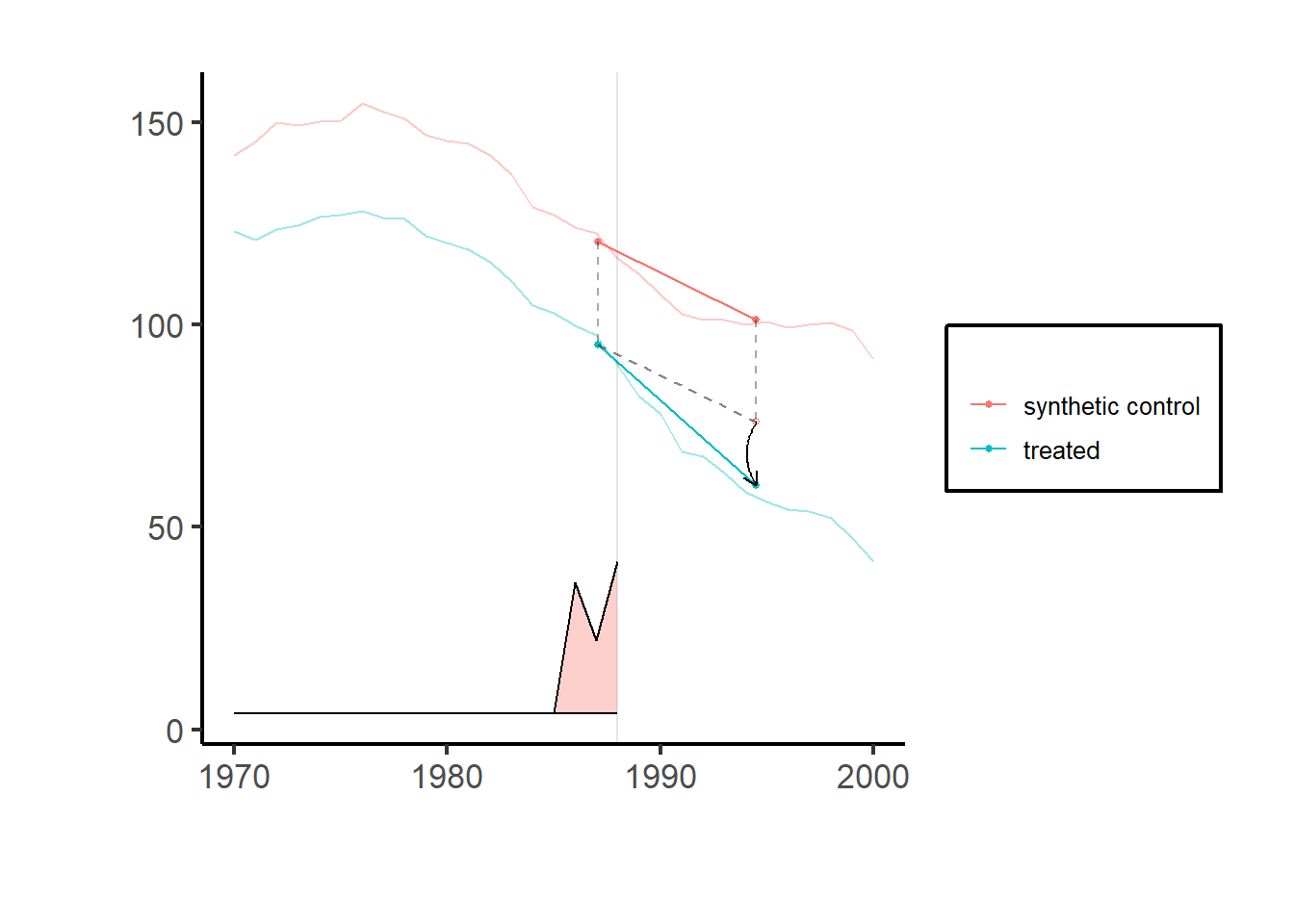
setup = synthdid::panel.matrices(synthdid::california_prop99)

# Run for specific estimators
results_selected = causalverse::panel_estimate(setup,
                                               selected_estimators = c("synthdid", "did", "sc"))

results_selected
#> $synthdid
#> $synthdid$estimate
#> synthdid: -15.604 +- NA. Effective N0/N0 = 16.4/38~0.4. Effective T0/T0 = 2.8/19~0.1. N1,T1 = 1,12.
#>
#> $synthdid$std.error
#> [1] 10.05324
#>
#>
#> $did
#> $did$estimate
#> synthdid: -27.349 +- NA. Effective N0/N0 = 38.0/38~1.0. Effective T0/T0 = 19.0/19~1.0. N1,T1 = 1,12.
#>
#> $did$std.error
#> [1] 15.81479
#>
#>
#> $sc
#> $sc$estimate
#> synthdid: -19.620 +- NA. Effective N0/N0 = 3.8/38~0.1. Effective T0/T0 = Inf/19~Inf. N1,T1 = 1,12.
#>
#> $sc$std.error
#> [1] 11.16422

# to access more details in the estimate object
summary(results_selected$did$estimate)
#> $estimate
#> [1] -27.34911
#>
#> $se
#>      [,1]
#> [1,]   NA
#>
#> $controls
#>                estimate 1
#> Wyoming             0.026
#> Wisconsin           0.026
#> West Virginia       0.026
#> Virginia            0.026
#> Vermont             0.026
#> Utah                0.026
#> Texas               0.026
#> Tennessee           0.026
#> South Dakota        0.026
#> South Carolina      0.026
#> Rhode Island        0.026
#> Pennsylvania        0.026
#> Oklahoma            0.026
#> Ohio                0.026
#> North Dakota        0.026
#> North Carolina      0.026
#> New Mexico          0.026
#> New Hampshire       0.026
#> Nevada              0.026
#> Nebraska            0.026
#> Montana             0.026
#> Missouri            0.026
#> Mississippi         0.026
#> Minnesota           0.026
#> Maine               0.026
#> Louisiana           0.026
#> Kentucky            0.026
#> Kansas              0.026
#> Iowa                0.026
#> Indiana             0.026
#> Illinois            0.026
#> Idaho               0.026
#> Georgia             0.026
#> Delaware            0.026
#> Connecticut         0.026
#>
#> $periods
#>      estimate 1
#> 1988      0.053
#> 1987      0.053
#> 1986      0.053
#> 1985      0.053
#> 1984      0.053
#> 1983      0.053
#> 1982      0.053
#> 1981      0.053
#> 1980      0.053
#> 1979      0.053
#> 1978      0.053
#> 1977      0.053
#> 1976      0.053
#> 1975      0.053
#> 1974      0.053
#> 1973      0.053
#> 1972      0.053
#> 1971      0.053
#>
#> $dimensions
#>           N1           N0 N0.effective           T1           T0 T0.effective
#>            1           38           38           12           19           19

causalverse::process_panel_estimate(results_selected)
#>     Method Estimate    SE
#> 1 SYNTHDID   -15.60 10.05
#> 2      DID   -27.35 15.81
#> 3       SC   -19.62 11.16
25.2.2 Staggered Adoption
To apply to staggered adoption settings using the SDID estimator (see examples in Arkhangelsky et al. (2021), p. 4115 similar to Ben-Michael, Feller, and Rothstein (2022)), we can:
Apply the SDID estimator repeatedly, once for every adoption date.
Using Ben-Michael, Feller, and Rothstein (2022) ’s method, form matrices for each adoption date. Apply SDID and average based on treated unit/time-period fractions.
Create multiple samples by splitting the data up by time periods. Each sample should have a consistent adoption date.
For a formal note on this special case, see Porreca (2022). It compares the outcomes from using SynthDiD with those from other estimators:
Two-Way Fixed Effects (TWFE),
The group time average treatment effect estimator from Callaway and Sant’Anna (2021),
The partially pooled synthetic control method estimator from Ben-Michael, Feller, and Rothstein (2021), in a staggered treatment adoption context.
-
The findings reveal that SynthDiD produces a different estimate of the average treatment effect compared to the other methods.
- Simulation results suggest that these differences could be due to the SynthDiD’s data generating process assumption (a latent factor model) aligning more closely with the actual data than the additive fixed effects model assumed by traditional DiD methods.
To explore heterogeneity of treatment effect, we can do subgroup analysis (Berman and Israeli 2022, 1092)
| Method | Advantages | Disadvantages | Procedure |
|---|---|---|---|
| Split Data into Subsets | Compares treated units to control units within the same subgroup. | Each subset uses a different synthetic control, making it challenging to compare effects across subgroups. |
|
| Control Group Comprising All Non-adopters | Control weights match pretrends well for each treated subgroup. | Each control unit receives a different weight for each treatment subgroup, making it difficult to compare results due to varying synthetic controls. |
|
| Use All Data to Estimate Synthetic Control Weights (recommend) | All units have the same synthetic control. | Pretrend match may not be as accurate since it aims to match the average outcome of all treated units, not just a specific subgroup. |
|
library(tidyverse)
df <- fixest::base_stagg |>
   dplyr::mutate(treatvar = if_else(time_to_treatment >= 0, 1, 0)) |>
   dplyr::mutate(treatvar = as.integer(if_else(year_treated > (5 + 2), 0, treatvar)))


est <- causalverse::synthdid_est_ate(
  data               = df,
  adoption_cohorts   = 5:7,
  lags               = 2,
  leads              = 2,
  time_var           = "year",
  unit_id_var        = "id",
  treated_period_var = "year_treated",
  treat_stat_var     = "treatvar",
  outcome_var        = "y"
)
#> adoption_cohort: 5
#> Treated units: 5 Control units: 65
#> adoption_cohort: 6
#> Treated units: 5 Control units: 60
#> adoption_cohort: 7
#> Treated units: 5 Control units: 55

data.frame(
    Period = names(est$TE_mean_w),
    ATE    = est$TE_mean_w,
    SE     = est$SE_mean_w
) |>
    causalverse::nice_tab()
#>    Period   ATE   SE
#> 1      -2 -0.05 0.22
#> 2      -1  0.05 0.22
#> 3       0 -5.07 0.80
#> 4       1 -4.68 0.51
#> 5       2 -3.70 0.79
#> 6 cumul.0 -5.07 0.80
#> 7 cumul.1 -4.87 0.55
#> 8 cumul.2 -4.48 0.53


causalverse::synthdid_plot_ate(est)
est_sub <- causalverse::synthdid_est_ate(
  data               = df,
  adoption_cohorts   = 5:7,
  lags               = 2,
  leads              = 2,
  time_var           = "year",
  unit_id_var        = "id",
  treated_period_var = "year_treated",
  treat_stat_var     = "treatvar",
  outcome_var        = "y",
  # a vector of subgroup id (from unit id)
  subgroup           =  c(
    # some are treated
    "11", "30", "49" ,
    # some are control within this period
    "20", "25", "21")
)
#> adoption_cohort: 5
#> Treated units: 3 Control units: 65
#> adoption_cohort: 6
#> Treated units: 0 Control units: 60
#> adoption_cohort: 7
#> Treated units: 0 Control units: 55

data.frame(
    Period = names(est_sub$TE_mean_w),
    ATE = est_sub$TE_mean_w,
    SE = est_sub$SE_mean_w
) |>
    causalverse::nice_tab()
#>    Period   ATE   SE
#> 1      -2  0.32 0.44
#> 2      -1 -0.32 0.44
#> 3       0 -4.29 1.68
#> 4       1 -4.00 1.52
#> 5       2 -3.44 2.90
#> 6 cumul.0 -4.29 1.68
#> 7 cumul.1 -4.14 1.52
#> 8 cumul.2 -3.91 1.82

causalverse::synthdid_plot_ate(est)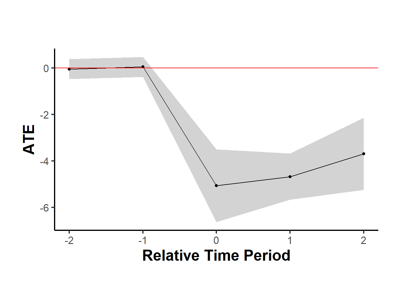
Plot different estimators
library(causalverse)
methods <- c("synthdid", "did", "sc", "sc_ridge", "difp", "difp_ridge")

estimates <- lapply(methods, function(method) {
  synthdid_est_ate(
    data               = df,
    adoption_cohorts   = 5:7,
    lags               = 2,
    leads              = 2,
    time_var           = "year",
    unit_id_var        = "id",
    treated_period_var = "year_treated",
    treat_stat_var     = "treatvar",
    outcome_var        = "y",
    method = method
  )
})

plots <- lapply(seq_along(estimates), function(i) {
  causalverse::synthdid_plot_ate(estimates[[i]],
                                 title = methods[i],
                                 theme = causalverse::ama_theme(base_size = 6))
})

gridExtra::grid.arrange(grobs = plots, ncol = 2)