15 Marginal Effects
In cases without polynomials or interactions, it can be easy to interpret the marginal effect.
For example,
\[ Y = \beta_1 X_1 + \beta_2 X_2 \]
where \(\beta\) are the marginal effects.
Numerical derivation is easier than analytical derivation.
- We need to choose values for all the variables to calculate the marginal effect of \(X\)
Analytical derivation
\[ f'(x) \equiv \lim_{h \to 0} \frac{f(x+h) - f(x)}{h} \]
E.g., \(f(x) = X^2\)
\[ \begin{aligned} f'(x) &= \lim_{h \to 0} \frac{(x+h)^2 - x^2}{h} \\ &= \frac{x^2 + 2xh + h^2 - x^2}{h} \\ &= \frac{2xh + h^2}{h} \\ &= 2x + h \\ &= 2x \end{aligned} \]
For numerically approach, we “just” need to find a small \(h\) to plug in our function. However, you also need a large enough \(h\) to have numerically accurate computation (Gould, Pitblado, and Poi 2010, chap. 1)
Numerically approach
One-sided derivative
\[ \begin{aligned} f'(x) &= \lim_{h \to 0} \frac{(x+h)^2 - x^2}{h} \\ & \approx \frac{f(x+h) -f(x)}{h} \end{aligned} \]
Alternatively, two-sided derivative
\[ f'_2(x) \approx \frac{f(x+h) - f(x- h)}{2h} \]
Marginal effects for
discrete variables (also known as incremental effects) are the change in \(E[Y|X]\) for a one unit change in \(X\)
continuous variables are the change in \(E[Y|X]\) for very small changes in \(X\) (not unit changes), because it’s a derivative, which is a limit when \(h \to 0\)
| Analytical derivation | Numerical derivation | |
|---|---|---|
| Marginal Effects | Rules of expectations | Approximate analytical solution |
| Standard Errors | Rules of variances | Delta method using the asymptotic errors (vcov matrix) |
15.1 Delta Method
- approximate the mean and variance of a function of random variables using a first-order Taylor approximation
- A semi-parametric method
- Alternative approaches:
Analytically derive a probability function for the margin
Simulation/Bootstrapping
- Resources:
Advanced: modmarg
Intermediate: UCLA stat
Simple: Another one
Let \(G(\beta)\) be a function of the parameters \(\beta\), then
\[ var(G(\beta)) \approx \nabla G(\beta) cov (\beta) \nabla G(\beta)' \]
where
- \(\nabla G(\beta)\) = the gradient of the partial derivatives of \(G(\beta)\) (also known as the Jacobian)
15.2 Average Marginal Effect Algorithm
For one-sided derivative \(\frac{\partial p(\mathbf{X},\beta)}{\partial X}\) in the probability scale
- Estimate your model
- For each observation \(i\)
Calculate \(\hat{Y}_{i0}\) which is the prediction in the probability scale using observed values
-
Increase \(X\) (variable of interest) by a “small” amount \(h\) (\(X_{new} = X + h\))
When \(X\) is continuous, \(h = (|\bar{X}| + 0.001) \times 0.001\) where \(\bar{X}\) is the mean value of \(X\)
When \(X\) is discrete, \(h = 1\)
Calculate \(\hat{Y}_{i1}\) which is the prediction in the probability scale using new \(X\) and other variables’ observed vales.
Calculate the difference between the two predictions as fraction of \(h\): \(\frac{\bar{Y}_{i1} - \bar{Y}_{i0}}{h}\)
- Average numerical derivative is \(E[\frac{\bar{Y}_{i1} - \bar{Y}_{i0}}{h}] \approx \frac{\partial p (Y|\mathbf{X}, \beta)}{\partial X}\)
Two-sided derivatives
- Estimate your model
- For each observation \(i\)
Calculate \(\hat{Y}_{i0}\) which is the prediction in the probability scale using observed values
-
Increase \(X\) (variable of interest) by a “small” amount \(h\) (\(X_{1} = X + h\)) and decrease \(X\) (variable of interest) by a “small” amount \(h\) (\(X_{2} = X - h\))
When \(X\) is continuous, \(h = (|\bar{X}| + 0.001) \times 0.001\) where \(\bar{X}\) is the mean value of \(X\)
When \(X\) is discrete, \(h = 1\)
Calculate \(\hat{Y}_{i1}\) which is the prediction in the probability scale using new \(X_1\) and other variables’ observed vales.
Calculate \(\hat{Y}_{i2}\) which is the prediction in the probability scale using new \(X_2\) and other variables’ observed vales.
Calculate the difference between the two predictions as fraction of \(h\): \(\frac{\bar{Y}_{i1} - \bar{Y}_{i2}}{2h}\)
- Average numerical derivative is \(E[\frac{\bar{Y}_{i1} - \bar{Y}_{i2}}{2h}] \approx \frac{\partial p (Y|\mathbf{X}, \beta)}{\partial X}\)
library(margins)
library(tidyverse)

data("mtcars")
mod <- lm(mpg ~ cyl * disp * hp, data = mtcars)
margins::margins(mod) %>% summary()
#>  factor     AME     SE       z      p    lower   upper
#>     cyl -4.0592 3.7614 -1.0792 0.2805 -11.4313  3.3130
#>    disp -0.0350 0.0132 -2.6473 0.0081  -0.0610 -0.0091
#>      hp -0.0284 0.0185 -1.5348 0.1248  -0.0647  0.0079

# function for variable
get_mae <- function(mod, var = "disp") {
    data = mod$model

    pred <- predict(mod)

    if (class(mod$model[[{
        {
            var
        }
    }]]) == "numeric") {
        h = (abs(mean(mod$model[[var]])) + 0.01) * 0.01
    } else {
        h = 1
    }

    data[[{
        {
            var
        }
    }]] <- data[[{
{
var
}
}]] - h

    pred_new <- predict(mod, newdata = data)

    mean(pred - pred_new) / h
}

get_mae(mod, var = "disp")
#> [1] -0.03504546
15.3 Packages
15.3.1 MarginalEffects
MarginalEffects package is a successor of margins and emtrends (faster, more efficient, more adaptable). Hence, this is advocated to be used.
- A limitation is that there is no readily function to correct for multiple comparisons. Hence, one can use the
p.adjustfunction to overcome this disadvantage.
Definitions from the package:
-
Marginal effects are slopes or derivatives (i.e., effect of changes in a variable on the outcome)
-
marginspackage defines marginal effects as “partial derivatives of the regression equation with respect to each variable in the model for each unit in the data.”
-
Marginal means are averages or integrals (i.e., marginalizing across rows of a prediction grid)
To customize your plot using plot_cme (which is a ggplot class), you can check this post by the author of the MarginalEffects package
Causal inference with the parametric g-formula
- Because the plug-in g estimator is equivalent to the average contrast in the
marginaleffectspackage.
To get predicted values
library(marginaleffects)
library(tidyverse)
data(mtcars)

mod <- lm(mpg ~ hp * wt * am, data = mtcars)
predictions(mod) %>% head()
#>
#>  Estimate Std. Error    z Pr(>|z|)     S 2.5 % 97.5 %
#>      22.5      0.884 25.4   <0.001 471.7  20.8   24.2
#>      20.8      1.194 17.4   <0.001 223.3  18.5   23.1
#>      25.3      0.709 35.7   <0.001 922.7  23.9   26.7
#>      20.3      0.704 28.8   <0.001 601.5  18.9   21.6
#>      17.0      0.712 23.9   <0.001 416.2  15.6   18.4
#>      19.7      0.875 22.5   <0.001 368.8  17.9   21.4
#>
#> Columns: rowid, estimate, std.error, statistic, p.value, s.value, conf.low, conf.high, mpg, hp, wt, am
# for specific reference values
predictions(mod, newdata = datagrid(am = 0, wt = c(2, 4)))
#>
#>  am wt Estimate Std. Error    z Pr(>|z|)     S 2.5 % 97.5 %  hp
#>   0  2     22.0       2.04 10.8   <0.001  87.4  18.0   26.0 147
#>   0  4     16.6       1.08 15.3   <0.001 173.8  14.5   18.7 147
#>
#> Columns: rowid, estimate, std.error, statistic, p.value, s.value, conf.low, conf.high, mpg, hp, am, wt
plot_cap(mod, condition = c("hp","wt"))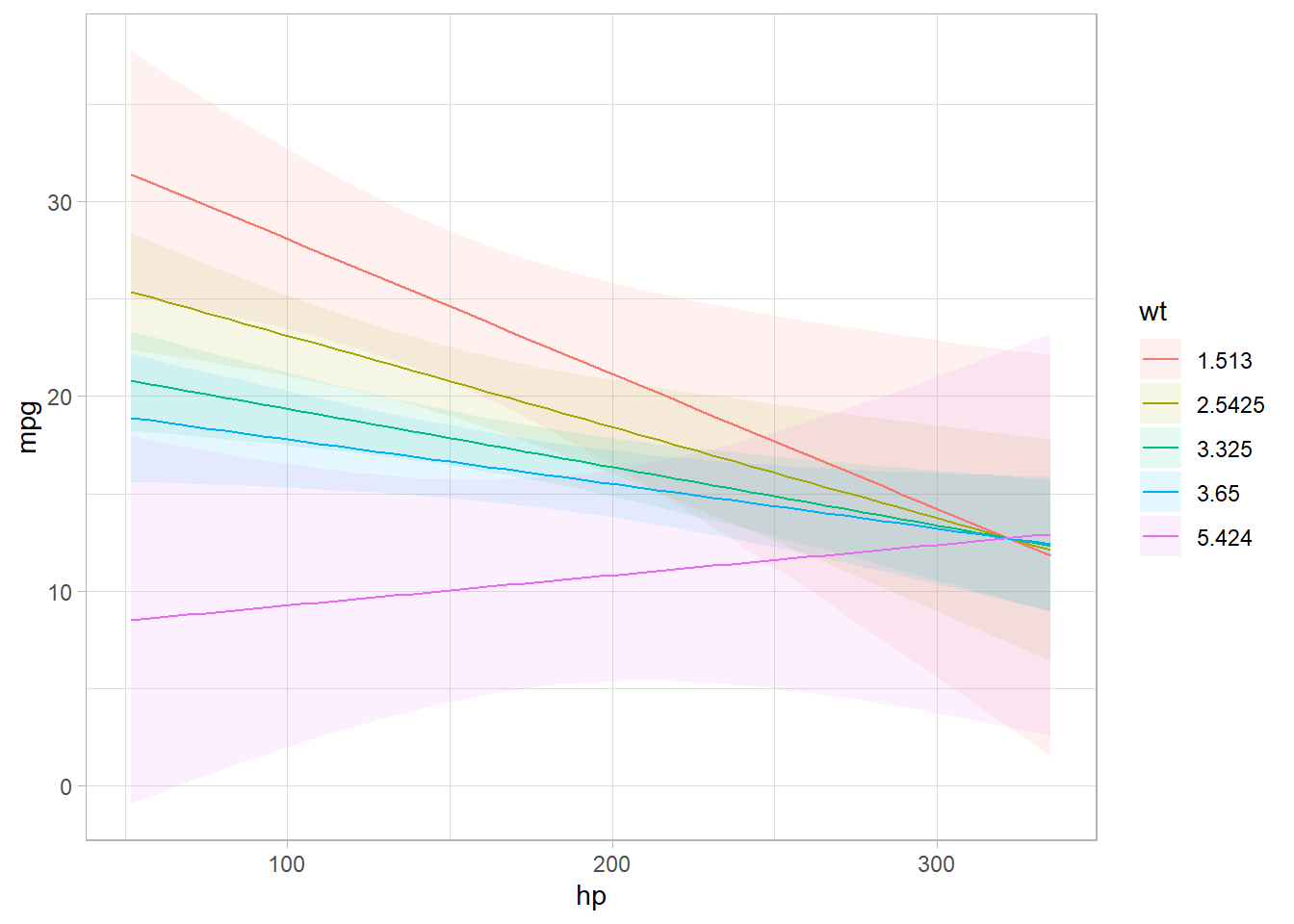
# Average Margianl Effects
mfx <- marginaleffects(mod, variables = c("hp", "wt"))
summary(mfx)
#>
#>  Term    Contrast Estimate Std. Error     z Pr(>|z|)   2.5 % 97.5 %
#>    hp mean(dY/dX)  -0.0381     0.0128 -2.98  0.00291 -0.0631 -0.013
#>    wt mean(dY/dX)  -3.9391     1.0858 -3.63  < 0.001 -6.0672 -1.811
#>
#> Columns: term, contrast, estimate, std.error, statistic, p.value, conf.low, conf.high

# Group-Average Marginal Effects
marginaleffects::marginaleffects(mod, by = "hp", variables = "am")
#>
#>  Term          Contrast  hp Estimate Std. Error      z Pr(>|z|)   S  2.5 %
#>    am mean(1) - mean(0)  52    3.976       5.20  0.764    0.445 1.2  -6.22
#>    am mean(1) - mean(0)  62   -2.774       2.51 -1.107    0.268 1.9  -7.68
#>    am mean(1) - mean(0)  65    2.999       4.13  0.725    0.468 1.1  -5.10
#>    am mean(1) - mean(0)  66    2.025       3.48  0.582    0.561 0.8  -4.80
#>    am mean(1) - mean(0)  91    1.858       2.76  0.674    0.500 1.0  -3.54
#>    am mean(1) - mean(0)  93    1.201       2.35  0.511    0.609 0.7  -3.40
#>    am mean(1) - mean(0)  95   -1.832       1.97 -0.931    0.352 1.5  -5.69
#>    am mean(1) - mean(0)  97    0.708       2.04  0.347    0.728 0.5  -3.28
#>    am mean(1) - mean(0) 105   -2.682       2.37 -1.132    0.258 2.0  -7.32
#>    am mean(1) - mean(0) 109   -0.237       1.59 -0.149    0.881 0.2  -3.35
#>    am mean(1) - mean(0) 110   -0.640       1.57 -0.407    0.684 0.5  -3.73
#>    am mean(1) - mean(0) 113    4.081       3.94  1.037    0.300 1.7  -3.63
#>    am mean(1) - mean(0) 123   -2.098       2.10 -0.998    0.318 1.7  -6.22
#>    am mean(1) - mean(0) 150   -1.429       1.90 -0.753    0.452 1.1  -5.15
#>    am mean(1) - mean(0) 175   -0.416       1.56 -0.266    0.790 0.3  -3.48
#>    am mean(1) - mean(0) 180   -1.381       2.47 -0.560    0.576 0.8  -6.22
#>    am mean(1) - mean(0) 205   -2.873       6.24 -0.460    0.645 0.6 -15.11
#>    am mean(1) - mean(0) 215   -2.534       6.95 -0.364    0.716 0.5 -16.16
#>    am mean(1) - mean(0) 230   -1.477       7.07 -0.209    0.835 0.3 -15.34
#>    am mean(1) - mean(0) 245    1.115       2.28  0.488    0.625 0.7  -3.36
#>    am mean(1) - mean(0) 264    2.106       2.29  0.920    0.358 1.5  -2.38
#>    am mean(1) - mean(0) 335    4.027       3.24  1.243    0.214 2.2  -2.32
#>  97.5 %
#>   14.18
#>    2.14
#>   11.10
#>    8.85
#>    7.26
#>    5.80
#>    2.02
#>    4.70
#>    1.96
#>    2.87
#>    2.45
#>   11.79
#>    2.02
#>    2.29
#>    2.64
#>    3.46
#>    9.36
#>   11.09
#>   12.39
#>    5.59
#>    6.59
#>   10.38
#>
#> Columns: term, contrast, hp, estimate, std.error, statistic, p.value, s.value, conf.low, conf.high, predicted_lo, predicted_hi, predicted

# Marginal effects at representative values
marginaleffects::marginaleffects(mod,
                                 newdata = datagrid(am = 0,
                                                    wt = c(2, 4)))
#>
#>  Term Contrast am wt Estimate Std. Error      z Pr(>|z|)   S   2.5 %   97.5 %
#>    am    1 - 0  0  2   2.5465     2.7860  0.914   0.3607 1.5 -2.9139  8.00694
#>    am    1 - 0  0  4  -2.9661     3.0381 -0.976   0.3289 1.6 -8.9207  2.98852
#>    hp    dY/dX  0  2  -0.0598     0.0283 -2.115   0.0344 4.9 -0.1153 -0.00439
#>    hp    dY/dX  0  4  -0.0309     0.0187 -1.654   0.0981 3.3 -0.0676  0.00572
#>    wt    dY/dX  0  2  -2.6762     1.4194 -1.885   0.0594 4.1 -5.4582  0.10587
#>    wt    dY/dX  0  4  -2.6762     1.4199 -1.885   0.0595 4.1 -5.4591  0.10676
#>
#> Columns: rowid, term, contrast, estimate, std.error, statistic, p.value, s.value, conf.low, conf.high, am, wt, predicted_lo, predicted_hi, predicted, mpg, hp

# Marginal Effects at the Mean
marginaleffects::marginaleffects(mod, newdata = "mean")
#>
#>  Term Contrast Estimate Std. Error      z Pr(>|z|)    S  2.5 %  97.5 %
#>    am    1 - 0  -0.8086    1.52383 -0.531  0.59568  0.7 -3.795  2.1781
#>    hp    dY/dX  -0.0323    0.00956 -3.375  < 0.001 10.4 -0.051 -0.0135
#>    wt    dY/dX  -3.7959    1.21310 -3.129  0.00175  9.2 -6.174 -1.4183
#>
#> Columns: rowid, term, contrast, estimate, std.error, statistic, p.value, s.value, conf.low, conf.high, predicted_lo, predicted_hi, predicted, mpg, hp, wt, am
# counterfactual
comparisons(mod, variables = list(am = 0:1)) %>% summary()
#>
#>  Term          Contrast Estimate Std. Error      z Pr(>|z|) 2.5 % 97.5 %
#>    am mean(1) - mean(0)  -0.0481       1.85 -0.026    0.979 -3.68   3.58
#>
#> Columns: term, contrast, estimate, std.error, statistic, p.value, conf.low, conf.high
15.3.2 margins
- Marginal effects are partial derivative of the regression equation with respect to each variable in the model for each unit in the data
Average Partial Effects: the contribution of each variable the outcome scale, conditional on the other variables involved in the link function transformation of the linear predictor
Average Marginal Effects: the marginal contribution of each variable on the scale of the linear predictor.
Average marginal effects are the mean of these unit-specific partial derivatives over some sample
margins package gives the marginal effects of models (a replication of the margins command in Stata).
prediction package gives the unit-specific and sample average predictions of models (similar to the predictive margins in Stata).
library(margins)

# examples by the package's authors
mod <- lm(mpg ~ cyl * hp + wt, data = mtcars)
summary(mod)
#>
#> Call:
#> lm(formula = mpg ~ cyl * hp + wt, data = mtcars)
#>
#> Residuals:
#>     Min      1Q  Median      3Q     Max
#> -3.3440 -1.4144 -0.6166  1.2160  4.2815
#>
#> Coefficients:
#>              Estimate Std. Error t value Pr(>|t|)
#> (Intercept) 52.017520   4.916935  10.579 4.18e-11 ***
#> cyl         -2.742125   0.800228  -3.427  0.00197 **
#> hp          -0.163594   0.052122  -3.139  0.00408 **
#> wt          -3.119815   0.661322  -4.718 6.51e-05 ***
#> cyl:hp       0.018954   0.006645   2.852  0.00823 **
#> ---
#> Signif. codes:  0 '***' 0.001 '**' 0.01 '*' 0.05 '.' 0.1 ' ' 1
#>
#> Residual standard error: 2.242 on 27 degrees of freedom
#> Multiple R-squared:  0.8795, Adjusted R-squared:  0.8616
#> F-statistic: 49.25 on 4 and 27 DF,  p-value: 5.065e-12
In cases where you have interaction or polynomial terms, the coefficient estimates cannot be interpreted as the marginal effects of X on Y. Hence, if you want to know the average marginal effects of each variable then
summary(margins(mod))
#>  factor     AME     SE       z      p   lower   upper
#>     cyl  0.0381 0.5999  0.0636 0.9493 -1.1376  1.2139
#>      hp -0.0463 0.0145 -3.1909 0.0014 -0.0748 -0.0179
#>      wt -3.1198 0.6613 -4.7176 0.0000 -4.4160 -1.8236

# equivalently
margins_summary(mod)
#>  factor     AME     SE       z      p   lower   upper
#>     cyl  0.0381 0.5999  0.0636 0.9493 -1.1376  1.2139
#>      hp -0.0463 0.0145 -3.1909 0.0014 -0.0748 -0.0179
#>      wt -3.1198 0.6613 -4.7176 0.0000 -4.4160 -1.8236

plot(margins(mod))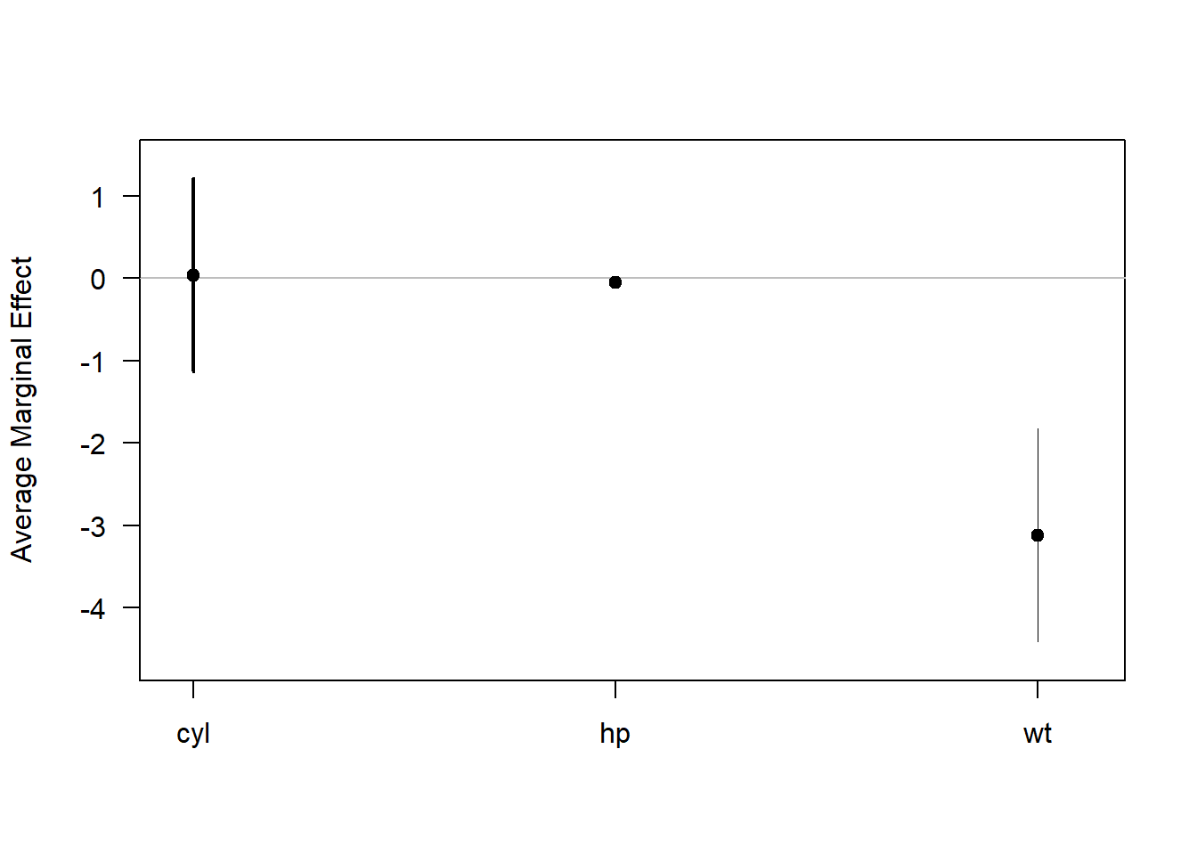
Marginal effects at the mean (MEM):
- Marginal effects at the mean values of the sample
- For discrete variables, it’s called average discrete change (ADC)
Average Marginal Effect (AME)
- An average of the marginal effects at each value of the sample
Marginal Effects at representative values (MER)
margins(mod, at = list(hp = 150))
#>  at(hp)    cyl       hp    wt
#>     150 0.1009 -0.04632 -3.12

margins(mod, at = list(hp = 150)) %>% summary()
#>  factor       hp     AME     SE       z      p   lower   upper
#>     cyl 150.0000  0.1009 0.6128  0.1647 0.8692 -1.1001  1.3019
#>      hp 150.0000 -0.0463 0.0145 -3.1909 0.0014 -0.0748 -0.0179
#>      wt 150.0000 -3.1198 0.6613 -4.7175 0.0000 -4.4160 -1.8236
15.3.3 mfx
Works well with Generalized Linear Models/glm package
For technical details, see the package vignette
| Model | Dependent Variable | Syntax |
|---|---|---|
| Probit | Binary | probitmfx |
| Logit | Binary | logitmfx |
| Poisson | Count | poissonmfx |
| Negative Binomial | Count | negbinmfx |
| Beta | Rate | betamfx |
library(mfx)
data("mtcars")
poissonmfx(formula = vs ~ mpg * cyl * disp, data = mtcars)
#> Call:
#> poissonmfx(formula = vs ~ mpg * cyl * disp, data = mtcars)
#>
#> Marginal Effects:
#>                    dF/dx   Std. Err.       z  P>|z|
#> mpg           1.4722e-03  8.7531e-03  0.1682 0.8664
#> cyl           6.6420e-03  3.9263e-02  0.1692 0.8657
#> disp          1.5899e-04  9.4555e-04  0.1681 0.8665
#> mpg:cyl      -3.4698e-04  2.0564e-03 -0.1687 0.8660
#> mpg:disp     -7.6794e-06  4.5545e-05 -0.1686 0.8661
#> cyl:disp     -3.3837e-05  1.9919e-04 -0.1699 0.8651
#> mpg:cyl:disp  1.6812e-06  9.8919e-06  0.1700 0.8650
This package can only give the marginal effect for each variable in the glm model, but not the average marginal effect that we might look for.