22 Multivariate Methods

\(y_1,...,y_p\) are possibly correlated random variables with means \(\mu_1,...,\mu_p\)

\[ \mathbf{y} = \left( \begin{array} {c} y_1 \\ . \\ y_p \\ \end{array} \right) \]

\[ E(\mathbf{y}) = \left( \begin{array} {c} \mu_1 \\ . \\ \mu_p \\ \end{array} \right) \]

Let \(\sigma_{ij} = cov(y_i, y_j)\) for \(i,j = 1,…,p\)

\[ \mathbf{\Sigma} = (\sigma_{ij}) = \left( \begin{array} {cccc} \sigma_{11} & \sigma_{22} & ... & \sigma_{1p} \\ \sigma_{21} & \sigma_{22} & ... & \sigma_{2p} \\ . & . & . & . \\ \sigma_{p1} & \sigma_{p2} & ... & \sigma_{pp} \end{array} \right) \]

where \(\mathbf{\Sigma}\) (symmetric) is the variance-covariance or dispersion matrix

Let \(\mathbf{u}_{p \times 1}\) and \(\mathbf{v}_{q \times 1}\) be random vectors with means \(\mu_u\) and \(\mu_v\) . Then

\[ \mathbf{\Sigma}_{uv} = cov(\mathbf{u,v}) = E[(\mathbf{u} - \mu_u)(\mathbf{v} - \mu_v)'] \]

in which \(\mathbf{\Sigma}_{uv} \neq \mathbf{\Sigma}_{vu}\) and \(\mathbf{\Sigma}_{uv} = \mathbf{\Sigma}_{vu}'\)

Properties of Covariance Matrices

1. Symmetric \(\mathbf{\Sigma}' = \mathbf{\Sigma}\)
2. Non-negative definite \(\mathbf{a'\Sigma a} \ge 0\) for any \(\mathbf{a} \in R^p\), which is equivalent to eigenvalues of \(\mathbf{\Sigma}\), \(\lambda_1 \ge \lambda_2 \ge ... \ge \lambda_p \ge 0\)
3. \(|\mathbf{\Sigma}| = \lambda_1 \lambda_2 ... \lambda_p \ge 0\) (generalized variance) (the bigger this number is, the more variation there is
4. \(trace(\mathbf{\Sigma}) = tr(\mathbf{\Sigma}) = \lambda_1 + ... + \lambda_p = \sigma_{11} + ... + \sigma_{pp} =\) sum of variance (total variance)

Note:

• \(\mathbf{\Sigma}\) is typically required to be positive definite, which means all eigenvalues are positive, and \(\mathbf{\Sigma}\) has an inverse \(\mathbf{\Sigma}^{-1}\) such that \(\mathbf{\Sigma}^{-1}\mathbf{\Sigma} = \mathbf{I}_{p \times p} = \mathbf{\Sigma \Sigma}^{-1}\)

Correlation Matrices

\[ \rho_{ij} = \frac{\sigma_{ij}}{\sqrt{\sigma_{ii} \sigma_{jj}}} \]

\[ \mathbf{R} = \left( \begin{array} {cccc} \rho_{11} & \rho_{12} & ... & \rho_{1p} \\ \rho_{21} & \rho_{22} & ... & \rho_{2p} \\ . & . & . &. \\ \rho_{p1} & \rho_{p2} & ... & \rho_{pp} \\ \end{array} \right) \]

where \(\rho_{ij}\) is the correlation, and \(\rho_{ii} = 1\) for all i

Alternatively,

\[ \mathbf{R} = [diag(\mathbf{\Sigma})]^{-1/2}\mathbf{\Sigma}[diag(\mathbf{\Sigma})]^{-1/2} \]

where \(diag(\mathbf{\Sigma})\) is the matrix which has the \(\sigma_{ii}\)’s on the diagonal and 0’s elsewhere

and \(\mathbf{A}^{1/2}\) (the square root of a symmetric matrix) is a symmetric matrix such as \(\mathbf{A} = \mathbf{A}^{1/2}\mathbf{A}^{1/2}\)

Equalities

Let

• \(\mathbf{x}\) and \(\mathbf{y}\) be random vectors with means \(\mu_x\) and \(\mu_y\) and variance -variance matrices \(\mathbf{\Sigma}_x\) and \(\mathbf{\Sigma}_y\).

• \(\mathbf{A}\) and \(\mathbf{B}\) be matrices of constants and \(\mathbf{c}\) and \(\mathbf{d}\) be vectors of constants

Then

• \(E(\mathbf{Ay + c} ) = \mathbf{A} \mu_y + c\)

• \(var(\mathbf{Ay + c}) = \mathbf{A} var(\mathbf{y})\mathbf{A}' = \mathbf{A \Sigma_y A}'\)

• \(cov(\mathbf{Ay + c, By+ d}) = \mathbf{A\Sigma_y B}'\)

• \(E(\mathbf{Ay + Bx + c}) = \mathbf{A \mu_y + B \mu_x + c}\)

• \(var(\mathbf{Ay + Bx + c}) = \mathbf{A \Sigma_y A' + B \Sigma_x B' + A \Sigma_{yx}B' + B\Sigma'_{yx}A'}\)

Multivariate Normal Distribution

Let \(\mathbf{y}\) be a multivariate normal (MVN) random variable with mean \(\mu\) and variance \(\mathbf{\Sigma}\). Then the density of \(\mathbf{y}\) is

\[ f(\mathbf{y}) = \frac{1}{(2\pi)^{p/2}|\mathbf{\Sigma}|^{1/2}} \exp(-\frac{1}{2} \mathbf{(y-\mu)'\Sigma^{-1}(y-\mu)} ) \]

\(\mathbf{y} \sim N_p(\mu, \mathbf{\Sigma})\)

22.0.1 Properties of MVN

• Let \(\mathbf{A}_{r \times p}\) be a fixed matrix. Then \(\mathbf{Ay} \sim N_r (\mathbf{A \mu, A \Sigma A'})\) . \(r \le p\) and all rows of \(\mathbf{A}\) must be linearly independent to guarantee that \(\mathbf{A \Sigma A}'\) is non-singular.

• Let \(\mathbf{G}\) be a matrix such that \(\mathbf{\Sigma}^{-1} = \mathbf{GG}'\). Then \(\mathbf{G'y} \sim N_p(\mathbf{G' \mu, I})\) and \(\mathbf{G'(y-\mu)} \sim N_p (0,\mathbf{I})\)

• Any fixed linear combination of \(y_1,...,y_p\) (say \(\mathbf{c'y}\)) follows \(\mathbf{c'y} \sim N_1 (\mathbf{c' \mu, c' \Sigma c})\)

• Define a partition, \([\mathbf{y}'_1,\mathbf{y}_2']'\) where

  • \(\mathbf{y}_1\) is \(p_1 \times 1\)

  • \(\mathbf{y}_2\) is \(p_2 \times 1\),

  • \(p_1 + p_2 = p\)

  • \(p_1,p_2 \ge 1\) Then

\[ \left( \begin{array} {c} \mathbf{y}_1 \\ \mathbf{y}_2 \\ \end{array} \right) \sim N \left( \left( \begin{array} {c} \mu_1 \\ \mu_2 \\ \end{array} \right), \left( \begin{array} {cc} \mathbf{\Sigma}_{11} & \mathbf{\Sigma}_{12} \\ \mathbf{\Sigma}_{21} & \mathbf{\Sigma}_{22}\\ \end{array} \right) \right) \]

• The marginal distributions of \(\mathbf{y}_1\) and \(\mathbf{y}_2\) are \(\mathbf{y}_1 \sim N_{p1}(\mathbf{\mu_1, \Sigma_{11}})\) and \(\mathbf{y}_2 \sim N_{p2}(\mathbf{\mu_2, \Sigma_{22}})\)

• Individual components \(y_1,...,y_p\) are all normally distributed \(y_i \sim N_1(\mu_i, \sigma_{ii})\)

• The conditional distribution of \(\mathbf{y}_1\) and \(\mathbf{y}_2\) is normal

  • \(\mathbf{y}_1 | \mathbf{y}_2 \sim N_{p1}(\mathbf{\mu_1 + \Sigma_{12} \Sigma_{22}^{-1}(y_2 - \mu_2),\Sigma_{11} - \Sigma_{12} \Sigma_{22}^{-1} \sigma_{21}})\)

    • In this formula, we see if we know (have info about) \(\mathbf{y}_2\), we can re-weight \(\mathbf{y}_1\) ’s mean, and the variance is reduced because we know more about \(\mathbf{y}_1\) because we know \(\mathbf{y}_2\)

  • which is analogous to \(\mathbf{y}_2 | \mathbf{y}_1\). And \(\mathbf{y}_1\) and \(\mathbf{y}_2\) are independently distrusted only if \(\mathbf{\Sigma}_{12} = 0\)

• If \(\mathbf{y} \sim N(\mathbf{\mu, \Sigma})\) and \(\mathbf{\Sigma}\) is positive definite, then \(\mathbf{(y-\mu)' \Sigma^{-1} (y - \mu)} \sim \chi^2_{(p)}\)

• If \(\mathbf{y}_i\) are independent \(N_p (\mathbf{\mu}_i , \mathbf{\Sigma}_i)\) random variables, then for fixed matrices \(\mathbf{A}_{i(m \times p)}\), \(\sum_{i=1}^k \mathbf{A}_i \mathbf{y}_i \sim N_m (\sum_{i=1}^{k} \mathbf{A}_i \mathbf{\mu}_i, \sum_{i=1}^k \mathbf{A}_i \mathbf{\Sigma}_i \mathbf{A}_i)\)

Multiple Regression

\[ \left( \begin{array} {c} Y \\ \mathbf{x} \end{array} \right) \sim N_{p+1} \left( \left[ \begin{array} {c} \mu_y \\ \mathbf{\mu}_x \end{array} \right] , \left[ \begin{array} {cc} \sigma^2_Y & \mathbf{\Sigma}_{yx} \\ \mathbf{\Sigma}_{yx} & \mathbf{\Sigma}_{xx} \end{array} \right] \right) \]

The conditional distribution of Y given x follows a univariate normal distribution with

\[ \begin{aligned} E(Y| \mathbf{x}) &= \mu_y + \mathbf{\Sigma}_{yx} \Sigma_{xx}^{-1} (\mathbf{x}- \mu_x) \\ &= \mu_y - \Sigma_{yx} \Sigma_{xx}^{-1}\mu_x + \Sigma_{yx} \Sigma_{xx}^{-1}\mathbf{x} \\ &= \beta_0 + \mathbf{\beta'x} \end{aligned} \]

where \(\beta = (\beta_1,...,\beta_p)' = \mathbf{\Sigma}_{xx}^{-1} \mathbf{\Sigma}_{yx}'\) (e.g., analogous to \(\mathbf{(x'x)^{-1}x'y}\) but not the same if we consider \(Y_i\) and \(\mathbf{x}_i\), \(i = 1,..,n\) and use the empirical covariance formula: \(var(Y|\mathbf{x}) = \sigma^2_Y - \mathbf{\Sigma_{yx}\Sigma^{-1}_{xx} \Sigma'_{yx}}\))

Samples from Multivariate Normal Populations

A random sample of size n, \(\mathbf{y}_1,.., \mathbf{y}_n\) from \(N_p (\mathbf{\mu}, \mathbf{\Sigma})\). Then

• Since \(\mathbf{y}_1,..., \mathbf{y}_n\) are iid, their sample mean, \(\bar{\mathbf{y}} = \sum_{i=1}^n \mathbf{y}_i/n \sim N_p (\mathbf{\mu}, \mathbf{\Sigma}/n)\). that is, \(\bar{\mathbf{y}}\) is an unbiased estimator of \(\mathbf{\mu}\)

• The \(p \times p\) sample variance-covariance matrix, \(\mathbf{S}\) is \(\mathbf{S} = \frac{1}{n-1}\sum_{i=1}^n (\mathbf{y}_i - \bar{\mathbf{y}})(\mathbf{y}_i - \bar{\mathbf{y}})' = \frac{1}{n-1} (\sum_{i=1}^n \mathbf{y}_i \mathbf{y}_i' - n \bar{\mathbf{y}}\bar{\mathbf{y}}')\)

  • where \(\mathbf{S}\) is symmetric, unbiased estimator of \(\mathbf{\Sigma}\) and has \(p(p+1)/2\) random variables.

• \((n-1)\mathbf{S} \sim W_p (n-1, \mathbf{\Sigma})\) is a Wishart distribution with n-1 degrees of freedom and expectation \((n-1) \mathbf{\Sigma}\). The Wishart distribution is a multivariate extension of the Chi-squared distribution.

• \(\bar{\mathbf{y}}\) and \(\mathbf{S}\) are independent

• \(\bar{\mathbf{y}}\) and \(\mathbf{S}\) are sufficient statistics. (All of the info in the data about \(\mathbf{\mu}\) and \(\mathbf{\Sigma}\) is contained in \(\bar{\mathbf{y}}\) and \(\mathbf{S}\) , regardless of sample size).

Large Sample Properties

\(\mathbf{y}_1,..., \mathbf{y}_n\) are a random sample from some population with mean \(\mathbf{\mu}\) and variance-covariance matrix \(\mathbf{\Sigma}\)

• \(\bar{\mathbf{y}}\) is a consistent estimator for \(\mu\)

• \(\mathbf{S}\) is a consistent estimator for \(\mathbf{\Sigma}\)

• Multivariate Central Limit Theorem: Similar to the univariate case, \(\sqrt{n}(\bar{\mathbf{y}} - \mu) \dot{\sim} N_p (\mathbf{0,\Sigma})\) where n is large relative to p (\(n \ge 25p\)), which is equivalent to \(\bar{\mathbf{y}} \dot{\sim} N_p (\mu, \mathbf{\Sigma}/n)\)

• Wald’s Theorem: \(n(\bar{\mathbf{y}} - \mu)' \mathbf{S}^{-1} (\bar{\mathbf{y}} - \mu)\) when n is large relative to p.

Maximum Likelihood Estimation for MVN

Suppose iid \(\mathbf{y}_1 ,... \mathbf{y}_n \sim N_p (\mu, \mathbf{\Sigma})\), the likelihood function for the data is

\[ \begin{aligned} L(\mu, \mathbf{\Sigma}) &= \prod_{j=1}^n (\frac{1}{(2\pi)^{p/2}|\mathbf{\Sigma}|^{1/2}} \exp(-\frac{1}{2}(\mathbf{y}_j -\mu)'\mathbf{\Sigma}^{-1})(\mathbf{y}_j -\mu)) \\ &= \frac{1}{(2\pi)^{np/2}|\mathbf{\Sigma}|^{n/2}} \exp(-\frac{1}{2} \sum_{j=1}^n(\mathbf{y}_j -\mu)'\mathbf{\Sigma}^{-1})(\mathbf{y}_j -\mu) \end{aligned} \]

Then, the MLEs are

\[ \hat{\mu} = \bar{\mathbf{y}} \]

\[ \hat{\mathbf{\Sigma}} = \frac{n-1}{n} \mathbf{S} \]

using derivatives of the log of the likelihood function with respect to \(\mu\) and \(\mathbf{\Sigma}\)

Properties of MLEs

• Invariance: If \(\hat{\theta}\) is the MLE of \(\theta\), then the MLE of \(h(\theta)\) is \(h(\hat{\theta})\) for any function h(.)

• Consistency: MLEs are consistent estimators, but they are usually biased

• Efficiency: MLEs are efficient estimators (no other estimator has a smaller variance for large samples)

• Asymptotic normality: Suppose that \(\hat{\theta}_n\) is the MLE for \(\theta\) based upon n independent observations. Then \(\hat{\theta}_n \dot{\sim} N(\theta, \mathbf{H}^{-1})\)

  • \(\mathbf{H}\) is the Fisher Information Matrix, which contains the expected values of the second partial derivatives fo the log-likelihood function. the (i,j)th element of \(\mathbf{H}\) is \(-E(\frac{\partial^2 l(\mathbf{\theta})}{\partial \theta_i \partial \theta_j})\)

  • we can estimate \(\mathbf{H}\) by finding the form determined above, and evaluate it at \(\theta = \hat{\theta}_n\)

• Likelihood ratio testing: for some null hypothesis, \(H_0\) we can form a likelihood ratio test

  • The statistic is: \(\Lambda = \frac{\max_{H_0}l(\mathbf{\mu}, \mathbf{\Sigma|Y})}{\max l(\mu, \mathbf{\Sigma | Y})}\)

  • For large n, \(-2 \log \Lambda \sim \chi^2_{(v)}\) where v is the number of parameters in the unrestricted space minus the number of parameters under \(H_0\)

Test of Multivariate Normality

• Check univariate normality for each trait (X) separately

  • Can check \[Normality Assessment\]

  • The good thing is that if any of the univariate trait is not normal, then the joint distribution is not normal (see again [m]). If a joint multivariate distribution is normal, then the marginal distribution has to be normal.

  • However, marginal normality of all traits does not imply joint MVN

  • Easily rule out multivariate normality, but not easy to prove it

• Mardia’s tests for multivariate normality

  • Multivariate skewness is\[ \beta_{1,p} = E[(\mathbf{y}- \mathbf{\mu})' \mathbf{\Sigma}^{-1} (\mathbf{x} - \mathbf{\mu})]^3 \]

  • where \(\mathbf{x}\) and \(\mathbf{y}\) are independent, but have the same distribution (note: \(\beta\) here is not regression coefficient)

  • Multivariate kurtosis is defined as

  • \[ \beta_{2,p} - E[(\mathbf{y}- \mathbf{\mu})' \mathbf{\Sigma}^{-1} (\mathbf{x} - \mathbf{\mu})]^2 \]

  • For the MVN distribution, we have \(\beta_{1,p} = 0\) and \(\beta_{2,p} = p(p+2)\)

  • For a sample of size n, we can estimate

    \[ \hat{\beta}_{1,p} = \frac{1}{n^2}\sum_{i=1}^n \sum_{j=1}^n g^2_{ij} \]

    \[ \hat{\beta}_{2,p} = \frac{1}{n} \sum_{i=1}^n g^2_{ii} \]

    • where \(g_{ij} = (\mathbf{y}_i - \bar{\mathbf{y}})' \mathbf{S}^{-1} (\mathbf{y}_j - \bar{\mathbf{y}})\). Note: \(g_{ii} = d^2_i\) where \(d^2_i\) is the Mahalanobis distance

  • (Mardia 1970) shows for large n

    \[ \kappa_1 = \frac{n \hat{\beta}_{1,p}}{6} \dot{\sim} \chi^2_{p(p+1)(p+2)/6} \]

    \[ \kappa_2 = \frac{\hat{\beta}_{2,p} - p(p+2)}{\sqrt{8p(p+2)/n}} \sim N(0,1) \]

    • Hence, we can use \(\kappa_1\) and \(\kappa_2\) to test the null hypothesis of MVN.

    • When the data are non-normal, normal theory tests on the mean are sensitive to \(\beta_{1,p}\) , while tests on the covariance are sensitive to \(\beta_{2,p}\)

• Alternatively, Doornik-Hansen test for multivariate normality (Doornik and Hansen 2008)

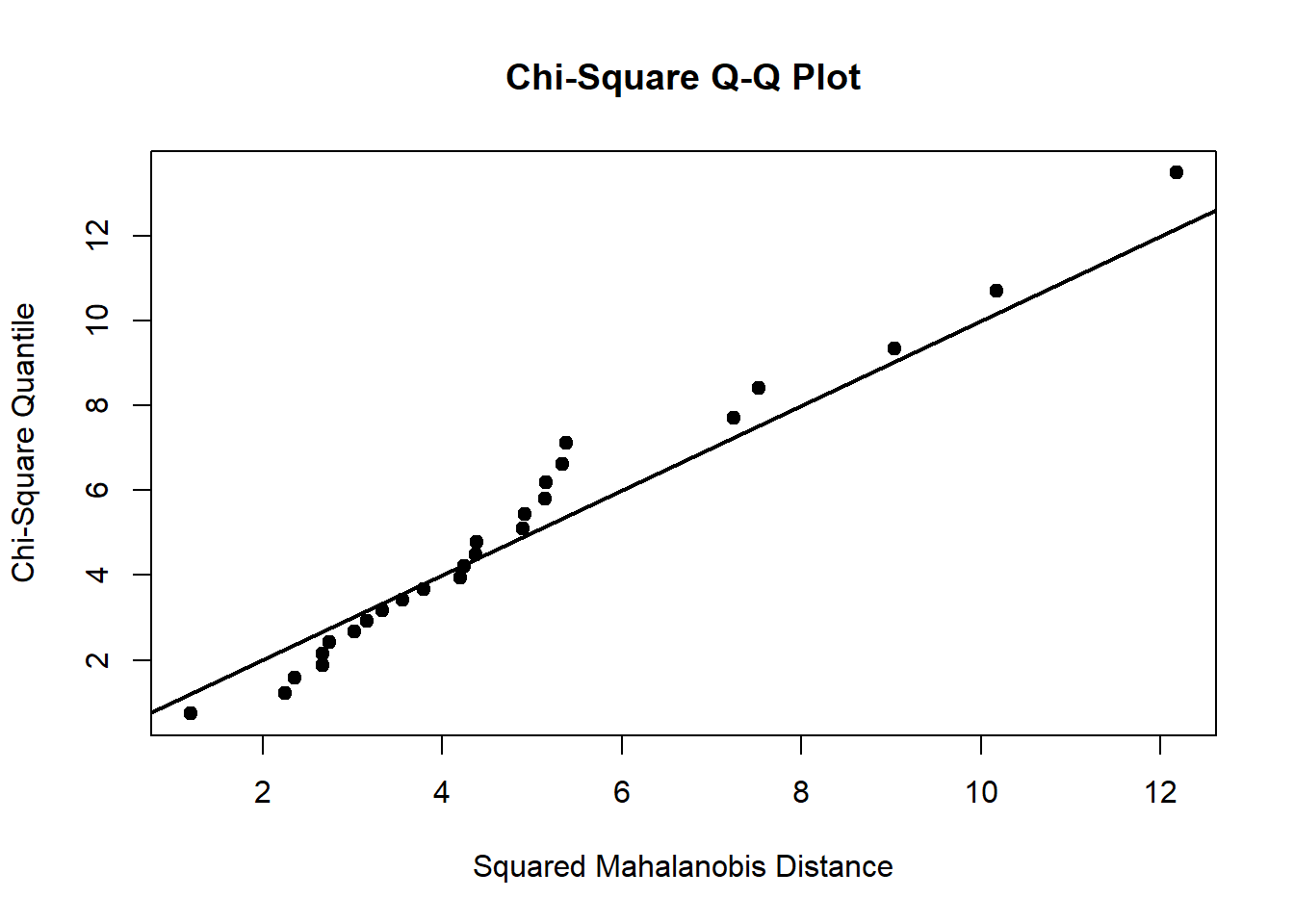
• Chi-square Q-Q plot

  • Let \(\mathbf{y}_i, i = 1,...,n\) be a random sample sample from \(N_p(\mathbf{\mu}, \mathbf{\Sigma})\)

  • Then \(\mathbf{z}_i = \mathbf{\Sigma}^{-1/2}(\mathbf{y}_i - \mathbf{\mu}), i = 1,...,n\) are iid \(N_p (\mathbf{0}, \mathbf{I})\). Thus, \(d_i^2 = \mathbf{z}_i' \mathbf{z}_i \sim \chi^2_p , i = 1,...,n\)

  • plot the ordered \(d_i^2\) values against the qualities of the \(\chi^2_p\) distribution. When normality holds, the plot should approximately resemble a straight lien passing through the origin at a 45 degree

  • it requires large sample size (i.e., sensitive to sample size). Even if we generate data from a MVN, the tail of the Chi-square Q-Q plot can still be out of line.

• If the data are not normal, we can

  • ignore it

  • use nonparametric methods

  • use models based upon an approximate distribution (e.g., GLMM)

  • try performing a transformation

library(heplots)
library(ICSNP)
library(MVN)
library(tidyverse)

trees = read.table("images/trees.dat")
names(trees) <- c("Nitrogen","Phosphorous","Potassium","Ash","Height")
str(trees)
#> 'data.frame':    26 obs. of  5 variables:
#>  $ Nitrogen   : num  2.2 2.1 1.52 2.88 2.18 1.87 1.52 2.37 2.06 1.84 ...
#>  $ Phosphorous: num  0.417 0.354 0.208 0.335 0.314 0.271 0.164 0.302 0.373 0.265 ...
#>  $ Potassium  : num  1.35 0.9 0.71 0.9 1.26 1.15 0.83 0.89 0.79 0.72 ...
#>  $ Ash        : num  1.79 1.08 0.47 1.48 1.09 0.99 0.85 0.94 0.8 0.77 ...
#>  $ Height     : int  351 249 171 373 321 191 225 291 284 213 ...

summary(trees)
#>     Nitrogen      Phosphorous       Potassium           Ash        
#>  Min.   :1.130   Min.   :0.1570   Min.   :0.3800   Min.   :0.4500  
#>  1st Qu.:1.532   1st Qu.:0.1963   1st Qu.:0.6050   1st Qu.:0.6375  
#>  Median :1.855   Median :0.2250   Median :0.7150   Median :0.9300  
#>  Mean   :1.896   Mean   :0.2506   Mean   :0.7619   Mean   :0.8873  
#>  3rd Qu.:2.160   3rd Qu.:0.2975   3rd Qu.:0.8975   3rd Qu.:0.9825  
#>  Max.   :2.880   Max.   :0.4170   Max.   :1.3500   Max.   :1.7900  
#>      Height     
#>  Min.   : 65.0  
#>  1st Qu.:122.5  
#>  Median :181.0  
#>  Mean   :196.6  
#>  3rd Qu.:276.0  
#>  Max.   :373.0
cor(trees, method = "pearson") # correlation matrix
#>              Nitrogen Phosphorous Potassium       Ash    Height
#> Nitrogen    1.0000000   0.6023902 0.5462456 0.6509771 0.8181641
#> Phosphorous 0.6023902   1.0000000 0.7037469 0.6707871 0.7739656
#> Potassium   0.5462456   0.7037469 1.0000000 0.6710548 0.7915683
#> Ash         0.6509771   0.6707871 0.6710548 1.0000000 0.7676771
#> Height      0.8181641   0.7739656 0.7915683 0.7676771 1.0000000

# qq-plot 
gg <- trees %>%
    pivot_longer(everything(), names_to = "Var", values_to = "Value") %>%
    ggplot(aes(sample = Value)) +
    geom_qq() +
    geom_qq_line() +
    facet_wrap("Var", scales = "free")
gg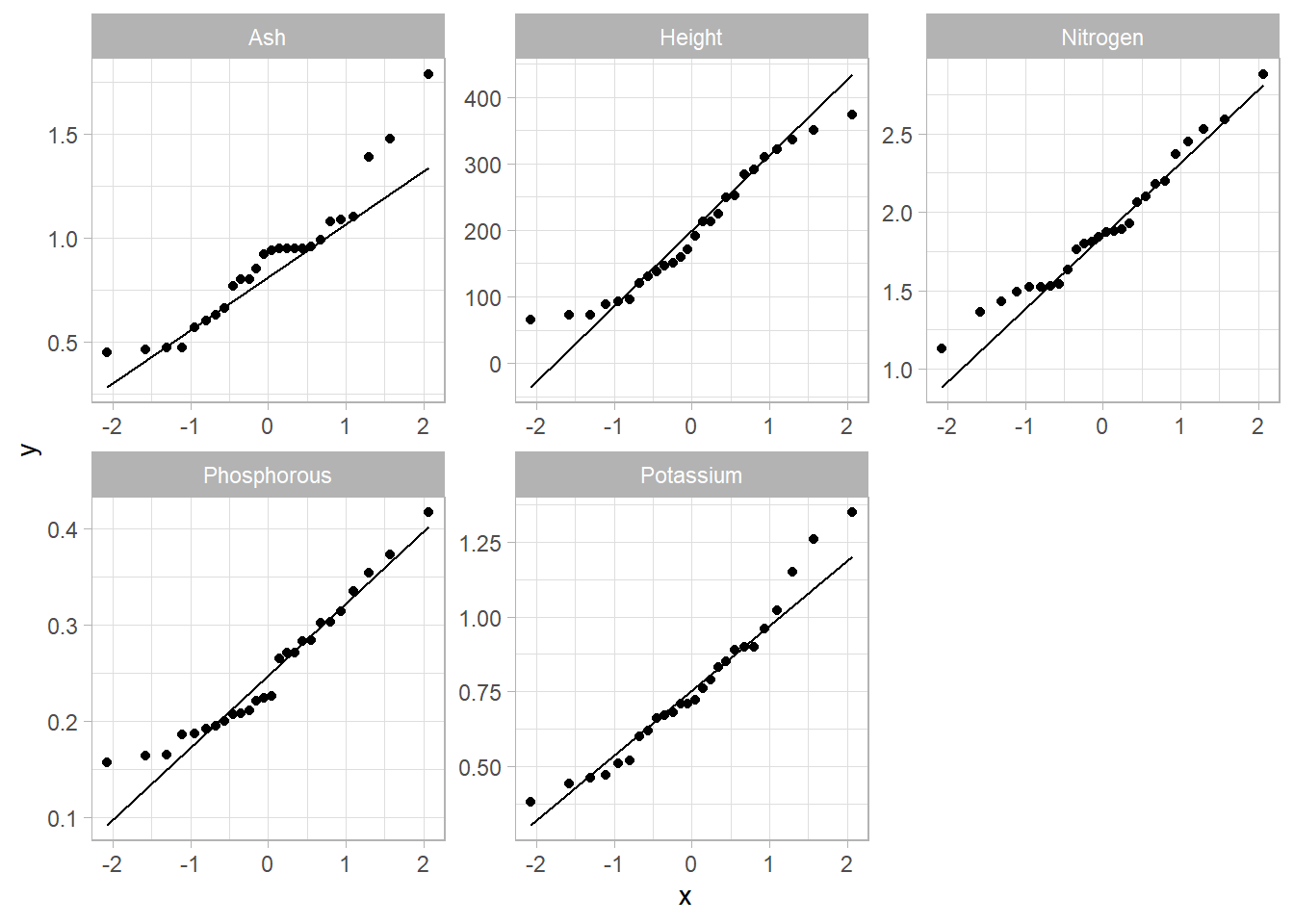

# Univariate normality
sw_tests <- apply(trees, MARGIN = 2, FUN = shapiro.test)
sw_tests
#> $Nitrogen
#> 
#>  Shapiro-Wilk normality test
#> 
#> data:  newX[, i]
#> W = 0.96829, p-value = 0.5794
#> 
#> 
#> $Phosphorous
#> 
#>  Shapiro-Wilk normality test
#> 
#> data:  newX[, i]
#> W = 0.93644, p-value = 0.1104
#> 
#> 
#> $Potassium
#> 
#>  Shapiro-Wilk normality test
#> 
#> data:  newX[, i]
#> W = 0.95709, p-value = 0.3375
#> 
#> 
#> $Ash
#> 
#>  Shapiro-Wilk normality test
#> 
#> data:  newX[, i]
#> W = 0.92071, p-value = 0.04671
#> 
#> 
#> $Height
#> 
#>  Shapiro-Wilk normality test
#> 
#> data:  newX[, i]
#> W = 0.94107, p-value = 0.1424
# Kolmogorov-Smirnov test 
ks_tests <- map(trees, ~ ks.test(scale(.x),"pnorm"))
ks_tests
#> $Nitrogen
#> 
#>  Asymptotic one-sample Kolmogorov-Smirnov test
#> 
#> data:  scale(.x)
#> D = 0.12182, p-value = 0.8351
#> alternative hypothesis: two-sided
#> 
#> 
#> $Phosphorous
#> 
#>  Asymptotic one-sample Kolmogorov-Smirnov test
#> 
#> data:  scale(.x)
#> D = 0.17627, p-value = 0.3944
#> alternative hypothesis: two-sided
#> 
#> 
#> $Potassium
#> 
#>  Asymptotic one-sample Kolmogorov-Smirnov test
#> 
#> data:  scale(.x)
#> D = 0.10542, p-value = 0.9348
#> alternative hypothesis: two-sided
#> 
#> 
#> $Ash
#> 
#>  Asymptotic one-sample Kolmogorov-Smirnov test
#> 
#> data:  scale(.x)
#> D = 0.14503, p-value = 0.6449
#> alternative hypothesis: two-sided
#> 
#> 
#> $Height
#> 
#>  Asymptotic one-sample Kolmogorov-Smirnov test
#> 
#> data:  scale(.x)
#> D = 0.1107, p-value = 0.9076
#> alternative hypothesis: two-sided

# Mardia's test, need large sample size for power
mardia_test <-
    mvn(
        trees,
        mvnTest = "mardia",
        covariance = FALSE,
        multivariatePlot = "qq"
    )

mardia_test$multivariateNormality
#>              Test         Statistic            p value Result
#> 1 Mardia Skewness  29.7248528871795   0.72054426745778    YES
#> 2 Mardia Kurtosis -1.67743173185383 0.0934580886477281    YES
#> 3             MVN              <NA>               <NA>    YES

# Doornik-Hansen's test 
dh_test <-
    mvn(
        trees,
        mvnTest = "dh",
        covariance = FALSE,
        multivariatePlot = "qq"
    )

dh_test$multivariateNormality
#>             Test        E df      p value MVN
#> 1 Doornik-Hansen 161.9446 10 1.285352e-29  NO

# Henze-Zirkler's test 
hz_test <-
    mvn(
        trees,
        mvnTest = "hz",
        covariance = FALSE,
        multivariatePlot = "qq"
    )
hz_test$multivariateNormality
#>            Test        HZ   p value MVN
#> 1 Henze-Zirkler 0.7591525 0.6398905 YES
# The last column indicates whether dataset follows a multivariate normality or not (i.e, YES or NO) at significance level 0.05.

# Royston's test
# can only apply for 3 < obs < 5000 (because of Shapiro-Wilk's test)
royston_test <-
    mvn(
        trees,
        mvnTest = "royston",
        covariance = FALSE,
        multivariatePlot = "qq"
    )
royston_test$multivariateNormality
#>      Test        H    p value MVN
#> 1 Royston 9.064631 0.08199215 YES


# E-statistic
estat_test <-
    mvn(
        trees,
        mvnTest = "energy",
        covariance = FALSE,
        multivariatePlot = "qq"
    )
estat_test$multivariateNormality
#>          Test Statistic p value MVN
#> 1 E-statistic  1.091101   0.532 YES

22.0.2 Mean Vector Inference

In the univariate normal distribution, we test \(H_0: \mu =\mu_0\) by using

\[ T = \frac{\bar{y}- \mu_0}{s/\sqrt{n}} \sim t_{n-1} \]

under the null hypothesis. And reject the null if \(|T|\) is large relative to \(t_{(1-\alpha/2,n-1)}\) because it means that seeing a value as large as what we observed is rare if the null is true

Equivalently,

\[ T^2 = \frac{(\bar{y}- \mu_0)^2}{s^2/n} = n(\bar{y}- \mu_0)(s^2)^{-1}(\bar{y}- \mu_0) \sim f_{(1,n-1)} \]

22.0.2.1 Natural Multivariate Generalization

\[ \begin{aligned} &H_0: \mathbf{\mu} = \mathbf{\mu}_0 \\ &H_a: \mathbf{\mu} \neq \mathbf{\mu}_0 \end{aligned} \]

Define Hotelling’s \(T^2\) by

\[ T^2 = n(\bar{\mathbf{y}} - \mathbf{\mu}_0)'\mathbf{S}^{-1}(\bar{\mathbf{y}} - \mathbf{\mu}_0) \]

which can be viewed as a generalized distance between \(\bar{\mathbf{y}}\) and \(\mathbf{\mu}_0\)

Under the assumption of normality,

\[ F = \frac{n-p}{(n-1)p} T^2 \sim f_{(p,n-p)} \]

and reject the null hypothesis when \(F > f_{(1-\alpha, p, n-p)}\)

• The \(T^2\) test is invariant to changes in measurement units.

  • If \(\mathbf{z = Cy + d}\) where \(\mathbf{C}\) and \(\mathbf{d}\) do not depend on \(\mathbf{y}\), then \(T^2(\mathbf{z}) - T^2(\mathbf{y})\)

• The \(T^2\) test can be derived as a likelihood ratio test of \(H_0: \mu = \mu_0\)

22.0.2.2 Confidence Intervals

22.0.2.2.1 Confidence Region

An “exact” \(100(1-\alpha)\%\) confidence region for \(\mathbf{\mu}\) is the set of all vectors, \(\mathbf{v}\), which are “close enough” to the observed mean vector, \(\bar{\mathbf{y}}\) to satisfy

\[ n(\bar{\mathbf{y}} - \mathbf{\mu}_0)'\mathbf{S}^{-1}(\bar{\mathbf{y}} - \mathbf{\mu}_0) \le \frac{(n-1)p}{n-p} f_{(1-\alpha, p, n-p)} \]

• \(\mathbf{v}\) are just the mean vectors that are not rejected by the \(T^2\) test when \(\mathbf{\bar{y}}\) is observed.

In case that you have 2 parameters, the confidence region is a “hyper-ellipsoid”.

In this region, it consists of all \(\mathbf{\mu}_0\) vectors for which the \(T^2\) test would not reject \(H_0\) at significance level \(\alpha\)

Even though the confidence region better assesses the joint knowledge concerning plausible values of \(\mathbf{\mu}\) , people typically include confidence statement about the individual component means. We’d like all of the separate confidence statements to hold simultaneously with a specified high probability. Simultaneous confidence intervals: intervals against any statement being incorrect

22.0.2.2.1.1 Simultaneous Confidence Statements

• Intervals based on a rectangular confidence region by projecting the previous region onto the coordinate axes:

\[ \bar{y}_{i} \pm \sqrt{\frac{(n-1)p}{n-p}f_{(1-\alpha, p,n-p)}\frac{s_{ii}}{n}} \]

for all \(i = 1,..,p\)

which implied confidence region is conservative; it has at least \(100(1- \alpha)\%\)

Generally, simultaneous \(100(1-\alpha) \%\) confidence intervals for all linear combinations , \(\mathbf{a}\) of the elements of the mean vector are given by

\[ \mathbf{a'\bar{y}} \pm \sqrt{\frac{(n-1)p}{n-p}f_{(1-\alpha, p,n-p)}\frac{\mathbf{a'Sa}}{n}} \]

• works for any arbitrary linear combination \(\mathbf{a'\mu} = a_1 \mu_1 + ... + a_p \mu_p\), which is a projection onto the axis in the direction of \(\mathbf{a}\)

• These intervals have the property that the probability that at least one such interval does not contain the appropriate \(\mathbf{a' \mu}\) is no more than \(\alpha\)

• These types of intervals can be used for “data snooping” (like \[Scheffe\])

22.0.2.2.1.2 One \(\mu\) at a time

• One at a time confidence intervals:

\[ \bar{y}_i \pm t_{(1 - \alpha/2, n-1} \sqrt{\frac{s_{ii}}{n}} \]

• Each of these intervals has a probability of \(1-\alpha\) of covering the appropriate \(\mu_i\)

• But they ignore the covariance structure of the \(p\) variables

• If we only care about \(k\) simultaneous intervals, we can use “one at a time” method with the \[Bonferroni\] correction.

• This method gets more conservative as the number of intervals \(k\) increases.

22.0.3 General Hypothesis Testing

22.0.3.1 One-sample Tests

\[ H_0: \mathbf{C \mu= 0} \]

where

• \(\mathbf{C}\) is a \(c \times p\) matrix of rank c where \(c \le p\)

We can test this hypothesis using the following statistic

\[ F = \frac{n - c}{(n-1)c} T^2 \]

where \(T^2 = n(\mathbf{C\bar{y}})' (\mathbf{CSC'})^{-1} (\mathbf{C\bar{y}})\)

Example:

\[ H_0: \mu_1 = \mu_2 = ... = \mu_p \]

Equivalently,

\[ \begin{aligned} \mu_1 - \mu_2 &= 0 \\ &\vdots \\ \mu_{p-1} - \mu_p &= 0 \end{aligned} \]

a total of \(p-1\) tests. Hence, we have \(\mathbf{C}\) as the \(p - 1 \times p\) matrix

\[ \mathbf{C} = \left( \begin{array} {ccccc} 1 & -1 & 0 & \ldots & 0 \\ 0 & 1 & -1 & \ldots & 0 \\ \vdots & \vdots & \vdots & \ddots & \vdots \\ 0 & 0 & \ldots & 1 & -1 \end{array} \right) \]

number of rows = \(c = p -1\)

Equivalently, we can also compare all of the other means to the first mean. Then, we test \(\mu_1 - \mu_2 = 0, \mu_1 - \mu_3 = 0,..., \mu_1 - \mu_p = 0\), the \((p-1) \times p\) matrix \(\mathbf{C}\) is

\[ \mathbf{C} = \left( \begin{array} {ccccc} -1 & 1 & 0 & \ldots & 0 \\ -1 & 0 & 1 & \ldots & 0 \\ \vdots & \vdots & \vdots & \ddots & \vdots \\ -1 & 0 & \ldots & 0 & 1 \end{array} \right) \]

The value of \(T^2\) is invariant to these equivalent choices of \(\mathbf{C}\)

This is often used for repeated measures designs, where each subject receives each treatment once over successive periods of time (all treatments are administered to each unit).

Example:

Let \(y_{ij}\) be the response from subject i at time j for \(i = 1,..,n, j = 1,...,T\). In this case, \(\mathbf{y}_i = (y_{i1}, ..., y_{iT})', i = 1,...,n\) are a random sample from \(N_T (\mathbf{\mu}, \mathbf{\Sigma})\)

Let \(n=8\) subjects, \(T = 6\). We are interested in \(\mu_1, .., \mu_6\)

\[ H_0: \mu_1 = \mu_2 = ... = \mu_6 \]

Equivalently,

\[ \begin{aligned} \mu_1 - \mu_2 &= 0 \\ \mu_2 - \mu_3 &= 0 \\ &... \\ \mu_5 - \mu_6 &= 0 \end{aligned} \]

We can test orthogonal polynomials for 4 equally spaced time points. To test for example the null hypothesis that quadratic and cubic effects are jointly equal to 0, we would define \(\mathbf{C}\)

\[ \mathbf{C} = \left( \begin{array} {cccc} 1 & -1 & -1 & 1 \\ -1 & 3 & -3 & 1 \end{array} \right) \]

22.0.3.2 Two-Sample Tests

Consider the analogous two sample multivariate tests.

Example: we have data on two independent random samples, one sample from each of two populations

\[ \begin{aligned} \mathbf{y}_{1i} &\sim N_p (\mathbf{\mu_1, \Sigma}) \\ \mathbf{y}_{2j} &\sim N_p (\mathbf{\mu_2, \Sigma}) \end{aligned} \]

We assume

• normality

• equal variance-covariance matrices

• independent random samples

We can summarize our data using the sufficient statistics \(\mathbf{\bar{y}}_1, \mathbf{S}_1, \mathbf{\bar{y}}_2, \mathbf{S}_2\) with respective sample sizes, \(n_1,n_2\)

Since we assume that \(\mathbf{\Sigma}_1 = \mathbf{\Sigma}_2 = \mathbf{\Sigma}\), compute a pooled estimate of the variance-covariance matrix on \(n_1 + n_2 - 2\) df

\[ \mathbf{S} = \frac{(n_1 - 1)\mathbf{S}_1 + (n_2-1) \mathbf{S}_2}{(n_1 -1) + (n_2 - 1)} \]

\[ \begin{aligned} &H_0: \mathbf{\mu}_1 = \mathbf{\mu}_2 \\ &H_a: \mathbf{\mu}_1 \neq \mathbf{\mu}_2 \end{aligned} \]

At least one element of the mean vectors is different

We use

• \(\mathbf{\bar{y}}_1 - \mathbf{\bar{y}}_2\) to estimate \(\mu_1 - \mu_2\)

• \(\mathbf{S}\) to estimate \(\mathbf{\Sigma}\)

  Note: because we assume the two populations are independent, there is no covariance

  \(cov(\mathbf{\bar{y}}_1 - \mathbf{\bar{y}}_2) = var(\mathbf{\bar{y}}_1) + var(\mathbf{\bar{y}}_2) = \frac{\mathbf{\Sigma_1}}{n_1} + \frac{\mathbf{\Sigma_2}}{n_2} = \mathbf{\Sigma}(\frac{1}{n_1} + \frac{1}{n_2})\)

Reject \(H_0\) if

\[ \begin{aligned} T^2 &= (\mathbf{\bar{y}}_1 - \mathbf{\bar{y}}_2)'\{ \mathbf{S} (\frac{1}{n_1} + \frac{1}{n_2})\}^{-1} (\mathbf{\bar{y}}_1 - \mathbf{\bar{y}}_2)\\ &= \frac{n_1 n_2}{n_1 +n_2} (\mathbf{\bar{y}}_1 - \mathbf{\bar{y}}_2)'\{ \mathbf{S} \}^{-1} (\mathbf{\bar{y}}_1 - \mathbf{\bar{y}}_2)\\ & \ge \frac{(n_1 + n_2 -2)p}{n_1 + n_2 - p - 1} f_{(1- \alpha,n_1 + n_2 - p -1)} \end{aligned} \]

or equivalently, if

\[ F = \frac{n_1 + n_2 - p -1}{(n_1 + n_2 -2)p} T^2 \ge f_{(1- \alpha, p , n_1 + n_2 -p -1)} \]

A \(100(1-\alpha) \%\) confidence region for \(\mu_1 - \mu_2\) consists of all vector \(\delta\) which satisfy

\[ \frac{n_1 n_2}{n_1 + n_2} (\mathbf{\bar{y}}_1 - \mathbf{\bar{y}}_2 - \mathbf{\delta})' \mathbf{S}^{-1}(\mathbf{\bar{y}}_1 - \mathbf{\bar{y}}_2 - \mathbf{\delta}) \le \frac{(n_1 + n_2 - 2)p}{n_1 + n_2 -p - 1}f_{(1-\alpha, p , n_1 + n_2 - p -1)} \]

The simultaneous confidence intervals for all linear combinations of \(\mu_1 - \mu_2\) have the form

\[ \mathbf{a'}(\mathbf{\bar{y}}_1 - \mathbf{\bar{y}}_2) \pm \sqrt{\frac{(n_1 + n_2 -2)p}{n_1 + n_2 - p -1}}f_{(1-\alpha, p, n_1 + n_2 -p -1)} \times \sqrt{\mathbf{a'Sa}(\frac{1}{n_1} + \frac{1}{n_2})} \]

Bonferroni intervals, for k combinations

\[ (\bar{y}_{1i} - \bar{y}_{2i}) \pm t_{(1-\alpha/2k, n_1 + n_2 - 2)}\sqrt{(\frac{1}{n_1} + \frac{1}{n_2})s_{ii}} \]

22.0.3.3 Model Assumptions

If model assumption are not met

• Unequal Covariance Matrices

  • If \(n_1 = n_2\) (large samples) there is little effect on the Type I error rate and power fo the two sample test

  • If \(n_1 > n_2\) and the eigenvalues of \(\mathbf{\Sigma}_1 \mathbf{\Sigma}^{-1}_2\) are less than 1, the Type I error level is inflated

  • If \(n_1 > n_2\) and some eigenvalues of \(\mathbf{\Sigma}_1 \mathbf{\Sigma}_2^{-1}\) are greater than 1, the Type I error rate is too small, leading to a reduction in power

• Sample Not Normal

  • Type I error level of the two sample \(T^2\) test isn’t much affect by moderate departures from normality if the two populations being sampled have similar distributions

  • One sample \(T^2\) test is much more sensitive to lack of normality, especially when the distribution is skewed.

  • Intuitively, you can think that in one sample your distribution will be sensitive, but the distribution of the difference between two similar distributions will not be as sensitive.

  • Solutions:

    • Transform to make the data more normal

    • Large large samples, use the \(\chi^2\) (Wald) test, in which populations don’t need to be normal, or equal sample sizes, or equal variance-covariance matrices

      • \(H_0: \mu_1 - \mu_2 =0\) use \((\mathbf{\bar{y}}_1 - \mathbf{\bar{y}}_2)'( \frac{1}{n_1} \mathbf{S}_1 + \frac{1}{n_2}\mathbf{S}_2)^{-1}(\mathbf{\bar{y}}_1 - \mathbf{\bar{y}}_2) \dot{\sim} \chi^2_{(p)}\)

22.0.3.3.1 Equal Covariance Matrices Tests

With independent random samples from k populations of \(p\)-dimensional vectors. We compute the sample covariance matrix for each, \(\mathbf{S}_i\), where \(i = 1,...,k\)

\[ \begin{aligned} &H_0: \mathbf{\Sigma}_1 = \mathbf{\Sigma}_2 = \ldots = \mathbf{\Sigma}_k = \mathbf{\Sigma} \\ &H_a: \text{at least 2 are different} \end{aligned} \]

Assume \(H_0\) is true, we would use a pooled estimate of the common covariance matrix, \(\mathbf{\Sigma}\)

\[ \mathbf{S} = \frac{\sum_{i=1}^k (n_i -1)\mathbf{S}_i}{\sum_{i=1}^k (n_i - 1)} \]

with \(\sum_{i=1}^k (n_i -1)\)

22.0.3.3.1.1 Bartlett’s Test

(a modification of the likelihood ratio test). Define

\[ N = \sum_{i=1}^k n_i \]

and (note: \(| |\) are determinants here, not absolute value)

\[ M = (N - k) \log|\mathbf{S}| - \sum_{i=1}^k (n_i - 1) \log|\mathbf{S}_i| \]

\[ C^{-1} = 1 - \frac{2p^2 + 3p - 1}{6(p+1)(k-1)} \{\sum_{i=1}^k (\frac{1}{n_i - 1}) - \frac{1}{N-k} \} \]

• Reject \(H_0\) when \(MC^{-1} > \chi^2_{1- \alpha, (k-1)p(p+1)/2}\)

• If not all samples are from normal populations, \(MC^{-1}\) has a distribution which is often shifted to the right of the nominal \(\chi^2\) distribution, which means \(H_0\) is often rejected even when it is true (the Type I error level is inflated). Hence, it is better to test individual normality first, or then multivariate normality before you do Bartlett’s test.

22.0.3.4 Two-Sample Repeated Measurements

• Define \(\mathbf{y}_{hi} = (y_{hi1}, ..., y_{hit})'\) to be the observations from the i-th subject in the h-th group for times 1 through T

• Assume that \(\mathbf{y}_{11}, ..., \mathbf{y}_{1n_1}\) are iid \(N_t(\mathbf{\mu}_1, \mathbf{\Sigma})\) and that \(\mathbf{y}_{21},...,\mathbf{y}_{2n_2}\) are iid \(N_t(\mathbf{\mu}_2, \mathbf{\Sigma})\)

• \(H_0: \mathbf{C}(\mathbf{\mu}_1 - \mathbf{\mu}_2) = \mathbf{0}_c\) where \(\mathbf{C}\) is a \(c \times t\) matrix of rank \(c\) where \(c \le t\)

• The test statistic has the form

\[ T^2 = \frac{n_1 n_2}{n_1 + n_2} (\mathbf{\bar{y}}_1 - \mathbf{\bar{y}}_2)' \mathbf{C}'(\mathbf{CSC}')^{-1}\mathbf{C} (\mathbf{\bar{y}}_1 - \mathbf{\bar{y}}_2) \]

where \(\mathbf{S}\) is the pooled covariance estimate. Then,

\[ F = \frac{n_1 + n_2 - c -1}{(n_1 + n_2-2)c} T^2 \sim f_{(c, n_1 + n_2 - c-1)} \]

when \(H_0\) is true

If the null hypothesis \(H_0: \mu_1 = \mu_2\) is rejected. A weaker hypothesis is that the profiles for the two groups are parallel.

\[ \begin{aligned} \mu_{11} - \mu_{21} &= \mu_{12} - \mu_{22} \\ &\vdots \\ \mu_{1t-1} - \mu_{2t-1} &= \mu_{1t} - \mu_{2t} \end{aligned} \]

The null hypothesis matrix term is then

\(H_0: \mathbf{C}(\mu_1 - \mu_2) = \mathbf{0}_c\) , where \(c = t - 1\) and

\[ \mathbf{C} = \left( \begin{array} {ccccc} 1 & -1 & 0 & \ldots & 0 \\ 0 & 1 & -1 & \ldots & 0 \\ \vdots & \vdots & \vdots & \ddots & \vdots \\ 0 & 0 & 0 & \ldots & -1 \end{array} \right)_{(t-1) \times t} \]

# One-sample Hotelling's T^2 test
#  Create data frame
plants <- data.frame(
    y1 = c(2.11, 2.36, 2.13, 2.78, 2.17),
    y2 = c(10.1, 35.0, 2.0, 6.0, 2.0),
    y3 = c(3.4, 4.1, 1.9, 3.8, 1.7)
)

# Center the data with 
# the hypothesized means and make a matrix
plants_ctr <- plants %>%
    transmute(y1_ctr = y1 - 2.85,
              y2_ctr = y2 - 15.0,
              y3_ctr = y3 - 6.0) %>%
    as.matrix()

# Use anova.mlm to calculate Wilks' lambda
onesamp_fit <- anova(lm(plants_ctr ~ 1), test = "Wilks")
onesamp_fit
#> Analysis of Variance Table
#> 
#>             Df    Wilks approx F num Df den Df  Pr(>F)  
#> (Intercept)  1 0.054219   11.629      3      2 0.08022 .
#> Residuals    4                                          
#> ---
#> Signif. codes:  0 '***' 0.001 '**' 0.01 '*' 0.05 '.' 0.1 ' ' 1

can’t reject the null of hypothesized vector of means

# Paired-Sample Hotelling's T^2 test
library(ICSNP)

#  Create data frame
waste <- data.frame(
    case = 1:11,
    com_y1 = c(6, 6, 18, 8, 11, 34, 28, 71, 43, 33, 20),
    com_y2 = c(27, 23, 64, 44, 30, 75, 26, 124, 54, 30, 14),
    state_y1 = c(25, 28, 36, 35, 15, 44, 42, 54, 34, 29, 39),
    state_y2 = c(15, 13, 22, 29, 31, 64, 30, 64, 56, 20, 21)
)

# Calculate the difference between commercial and state labs
waste_diff <- waste %>%
    transmute(y1_diff = com_y1 - state_y1,
              y2_diff = com_y2 - state_y2)
# Run the test
paired_fit <- HotellingsT2(waste_diff)
# value T.2 in the output corresponds to 
# the approximate F-value in the output from anova.mlm
paired_fit 
#> 
#>  Hotelling's one sample T2-test
#> 
#> data:  waste_diff
#> T.2 = 6.1377, df1 = 2, df2 = 9, p-value = 0.02083
#> alternative hypothesis: true location is not equal to c(0,0)

reject the null that the two labs’ measurements are equal

# Independent-Sample Hotelling's T^2 test with Bartlett's test

# Read in data
steel <- read.table("images/steel.dat")
names(steel) <- c("Temp", "Yield", "Strength")
str(steel)
#> 'data.frame':    12 obs. of  3 variables:
#>  $ Temp    : int  1 1 1 1 1 2 2 2 2 2 ...
#>  $ Yield   : int  33 36 35 38 40 35 36 38 39 41 ...
#>  $ Strength: int  60 61 64 63 65 57 59 59 61 63 ...

# Plot the data
ggplot(steel, aes(x = Yield, y = Strength)) +
    geom_text(aes(label = Temp), size = 5) +
    geom_segment(aes(
        x = 33,
        y = 57.5,
        xend = 42,
        yend = 65
    ), col = "red")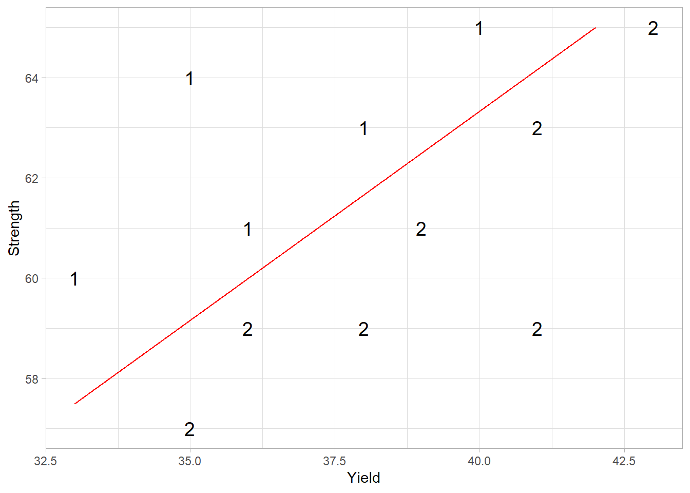

# Bartlett's test for equality of covariance matrices
# same thing as Box's M test in the multivariate setting
bart_test <- boxM(steel[, -1], steel$Temp)
bart_test # fail to reject the null of equal covariances 
#> 
#>  Box's M-test for Homogeneity of Covariance Matrices
#> 
#> data:  steel[, -1]
#> Chi-Sq (approx.) = 0.38077, df = 3, p-value = 0.9442

# anova.mlm
twosamp_fit <-
    anova(lm(cbind(Yield, Strength) ~ factor(Temp), 
             data = steel), 
          test = "Wilks")
twosamp_fit
#> Analysis of Variance Table
#> 
#>              Df    Wilks approx F num Df den Df    Pr(>F)    
#> (Intercept)   1 0.001177   3818.1      2      9 6.589e-14 ***
#> factor(Temp)  1 0.294883     10.8      2      9  0.004106 ** 
#> Residuals    10                                              
#> ---
#> Signif. codes:  0 '***' 0.001 '**' 0.01 '*' 0.05 '.' 0.1 ' ' 1

# ICSNP package
twosamp_fit2 <-
    HotellingsT2(cbind(steel$Yield, steel$Strength) ~ 
                     factor(steel$Temp))
twosamp_fit2
#> 
#>  Hotelling's two sample T2-test
#> 
#> data:  cbind(steel$Yield, steel$Strength) by factor(steel$Temp)
#> T.2 = 10.76, df1 = 2, df2 = 9, p-value = 0.004106
#> alternative hypothesis: true location difference is not equal to c(0,0)

reject null. Hence, there is a difference in the means of the bivariate normal distributions

22.1 MANOVA

Multivariate Analysis of Variance

One-way MANOVA

Compare treatment means for h different populations

Population 1: \(\mathbf{y}_{11}, \mathbf{y}_{12}, \dots, \mathbf{y}_{1n_1} \sim idd N_p (\mathbf{\mu}_1, \mathbf{\Sigma})\)

\(\vdots\)

Population h: \(\mathbf{y}_{h1}, \mathbf{y}_{h2}, \dots, \mathbf{y}_{hn_h} \sim idd N_p (\mathbf{\mu}_h, \mathbf{\Sigma})\)

Assumptions

1. Independent random samples from \(h\) different populations
2. Common covariance matrices
3. Each population is multivariate normal

Calculate the summary statistics \(\mathbf{\bar{y}}_i, \mathbf{S}\) and the pooled estimate of the covariance matrix \(\mathbf{S}\)

Similar to the univariate one-way ANVOA, we can use the effects model formulation \(\mathbf{\mu}_i = \mathbf{\mu} + \mathbf{\tau}_i\), where

• \(\mathbf{\mu}_i\) is the population mean for population i

• \(\mathbf{\mu}\) is the overall mean effect

• \(\mathbf{\tau}_i\) is the treatment effect of the i-th treatment.

For the one-way model: \(\mathbf{y}_{ij} = \mu + \tau_i + \epsilon_{ij}\) for \(i = 1,..,h; j = 1,..., n_i\) and \(\epsilon_{ij} \sim N_p(\mathbf{0, \Sigma})\)

However, the above model is over-parameterized (i.e., infinite number of ways to define \(\mathbf{\mu}\) and the \(\mathbf{\tau}_i\)’s such that they add up to \(\mu_i\). Thus we can constrain by having

\[ \sum_{i=1}^h n_i \tau_i = 0 \]

or

\[ \mathbf{\tau}_h = 0 \]

The observational equivalent of the effects model is

\[ \begin{aligned} \mathbf{y}_{ij} &= \mathbf{\bar{y}} + (\mathbf{\bar{y}}_i - \mathbf{\bar{y}}) + (\mathbf{y}_{ij} - \mathbf{\bar{y}}_i) \\ &= \text{overall sample mean} + \text{treatement effect} + \text{residual} \text{ (under univariate ANOVA)} \end{aligned} \]

After manipulation

\[ \sum_{i = 1}^h \sum_{j = 1}^{n_i} (\mathbf{\bar{y}}_{ij} - \mathbf{\bar{y}})(\mathbf{\bar{y}}_{ij} - \mathbf{\bar{y}})' = \sum_{i = 1}^h n_i (\mathbf{\bar{y}}_i - \mathbf{\bar{y}})(\mathbf{\bar{y}}_i - \mathbf{\bar{y}})' + \sum_{i=1}^h \sum_{j = 1}^{n_i} (\mathbf{\bar{y}}_{ij} - \mathbf{\bar{y}})(\mathbf{\bar{y}}_{ij} - \mathbf{\bar{y}}_i)' \]

LHS = Total corrected sums of squares and cross products (SSCP) matrix

RHS =

• 1st term = Treatment (or between subjects) sum of squares and cross product matrix (denoted H;B)

• 2nd term = residual (or within subject) SSCP matrix denoted (E;W)

Note:

\[ \mathbf{E} = (n_1 - 1)\mathbf{S}_1 + ... + (n_h -1) \mathbf{S}_h = (n-h) \mathbf{S} \]

MANOVA table

MONOVA table

Source	SSCP	df
Treatment	\(\mathbf{H}\)	\(h -1\)
Residual (error)	\(\mathbf{E}\)	\(\sum_{i= 1}^h n_i - h\)
Total Corrected	\(\mathbf{H + E}\)	\(\sum_{i=1}^h n_i -1\)

\[ H_0: \tau_1 = \tau_2 = \dots = \tau_h = \mathbf{0} \]

We consider the relative “sizes” of \(\mathbf{E}\) and \(\mathbf{H+E}\)

Wilk’s Lambda

Define Wilk’s Lambda

\[ \Lambda^* = \frac{|\mathbf{E}|}{|\mathbf{H+E}|} \]

Properties:

1. Wilk’s Lambda is equivalent to the F-statistic in the univariate case

2. The exact distribution of \(\Lambda^*\) can be determined for especial cases.

3. For large sample sizes, reject \(H_0\) if

\[ -(\sum_{i=1}^h n_i - 1 - \frac{p+h}{2}) \log(\Lambda^*) > \chi^2_{(1-\alpha, p(h-1))} \]

22.1.1 Testing General Hypotheses

• \(h\) different treatments

• with the i-th treatment

• applied to \(n_i\) subjects that

• are observed for \(p\) repeated measures.

Consider this a \(p\) dimensional obs on a random sample from each of \(h\) different treatment populations.

\[ \mathbf{y}_{ij} = \mathbf{\mu} + \mathbf{\tau}_i + \mathbf{\epsilon}_{ij} \]

for \(i = 1,..,h\) and \(j = 1,..,n_i\)

Equivalently,

\[ \mathbf{Y} = \mathbf{XB} + \mathbf{\epsilon} \]

where \(n = \sum_{i = 1}^h n_i\) and with restriction \(\mathbf{\tau}_h = 0\)

\[ \mathbf{Y}_{(n \times p)} = \left[ \begin{array} {c} \mathbf{y}_{11}' \\ \vdots \\ \mathbf{y}_{1n_1}' \\ \vdots \\ \mathbf{y}_{hn_h}' \end{array} \right], \mathbf{B}_{(h \times p)} = \left[ \begin{array} {c} \mathbf{\mu}' \\ \mathbf{\tau}_1' \\ \vdots \\ \mathbf{\tau}_{h-1}' \end{array} \right], \mathbf{\epsilon}_{(n \times p)} = \left[ \begin{array} {c} \epsilon_{11}' \\ \vdots \\ \epsilon_{1n_1}' \\ \vdots \\ \epsilon_{hn_h}' \end{array} \right] \]

\[ \mathbf{X}_{(n \times h)} = \left[ \begin{array} {ccccc} 1 & 1 & 0 & \ldots & 0 \\ \vdots & \vdots & \vdots & & \vdots \\ 1 & 1 & 0 & \ldots & 0 \\ \vdots & \vdots & \vdots & \ldots & \vdots \\ 1 & 0 & 0 & \ldots & 0 \\ \vdots & \vdots & \vdots & & \vdots \\ 1 & 0 & 0 & \ldots & 0 \end{array} \right] \]

Estimation

\[ \mathbf{\hat{B}} = (\mathbf{X'X})^{-1} \mathbf{X'Y} \]

Rows of \(\mathbf{Y}\) are independent (i.e., \(var(\mathbf{Y}) = \mathbf{I}_n \otimes \mathbf{\Sigma}\) , an \(np \times np\) matrix, where \(\otimes\) is the Kronecker product).

\[ \begin{aligned} &H_0: \mathbf{LBM} = 0 \\ &H_a: \mathbf{LBM} \neq 0 \end{aligned} \]

where

• \(\mathbf{L}\) is a \(g \times h\) matrix of full row rank (\(g \le h\)) = comparisons across groups

• \(\mathbf{M}\) is a \(p \times u\) matrix of full column rank (\(u \le p\)) = comparisons across traits

The general treatment corrected sums of squares and cross product is

\[ \mathbf{H} = \mathbf{M'Y'X(X'X)^{-1}L'[L(X'X)^{-1}L']^{-1}L(X'X)^{-1}X'YM} \]

or for the null hypothesis \(H_0: \mathbf{LBM} = \mathbf{D}\)

\[ \mathbf{H} = (\mathbf{\hat{LBM}} - \mathbf{D})'[\mathbf{X(X'X)^{-1}L}]^{-1}(\mathbf{\hat{LBM}} - \mathbf{D}) \]

The general matrix of residual sums of squares and cross product

\[ \mathbf{E} = \mathbf{M'Y'[I-X(X'X)^{-1}X']YM} = \mathbf{M'[Y'Y - \hat{B}'(X'X)^{-1}\hat{B}]M} \]

We can compute the following statistic eigenvalues of \(\mathbf{HE}^{-1}\)

• Wilk’s Criterion: \(\Lambda^* = \frac{|\mathbf{E}|}{|\mathbf{H} + \mathbf{E}|}\) . The df depend on the rank of \(\mathbf{L}, \mathbf{M}, \mathbf{X}\)

• Lawley-Hotelling Trace: \(U = tr(\mathbf{HE}^{-1})\)

• Pillai Trace: \(V = tr(\mathbf{H}(\mathbf{H}+ \mathbf{E}^{-1})\)

• Roy’s Maximum Root: largest eigenvalue of \(\mathbf{HE}^{-1}\)

If \(H_0\) is true and n is large, \(-(n-1- \frac{p+h}{2})\ln \Lambda^* \sim \chi^2_{p(h-1)}\). Some special values of p and h can give exact F-dist under \(H_0\)

# One-way MANOVA

library(car)
library(emmeans)
library(profileR)
library(tidyverse)

## Read in the data
gpagmat <- read.table("images/gpagmat.dat")

## Change the variable names
names(gpagmat) <- c("y1", "y2", "admit")

## Check the structure
str(gpagmat)
#> 'data.frame':    85 obs. of  3 variables:
#>  $ y1   : num  2.96 3.14 3.22 3.29 3.69 3.46 3.03 3.19 3.63 3.59 ...
#>  $ y2   : int  596 473 482 527 505 693 626 663 447 588 ...
#>  $ admit: int  1 1 1 1 1 1 1 1 1 1 ...


## Plot the data
gg <- ggplot(gpagmat, aes(x = y1, y = y2)) +
    geom_text(aes(label = admit, col = as.character(admit))) +
    scale_color_discrete(name = "Admission",
                         labels = c("Admit", "Do not admit", "Borderline")) +
    scale_x_continuous(name = "GPA") +
    scale_y_continuous(name = "GMAT")

## Fit one-way MANOVA
oneway_fit <- manova(cbind(y1, y2) ~ admit, data = gpagmat)
summary(oneway_fit, test = "Wilks")
#>           Df  Wilks approx F num Df den Df    Pr(>F)    
#> admit      1 0.6126   25.927      2     82 1.881e-09 ***
#> Residuals 83                                            
#> ---
#> Signif. codes:  0 '***' 0.001 '**' 0.01 '*' 0.05 '.' 0.1 ' ' 1

reject the null of equal multivariate mean vectors between the three admmission groups

# Repeated Measures MANOVA


## Create data frame
stress <- data.frame(
    subject = 1:8,
    begin = c(3, 2, 5, 6, 1, 5, 1, 5),
    middle = c(3, 4, 3, 7, 4, 7, 1, 2),
    final = c(6, 7, 4, 7, 6, 7, 3, 5)
)

• If independent = time with 3 levels -> univariate ANOVA (require sphericity assumption (i.e., the variances for all differences are equal))
• If each level of independent time as a separate variable -> MANOVA (does not require sphericity assumption)

## MANOVA
stress_mod <- lm(cbind(begin, middle, final) ~ 1, data = stress)
idata <-
    data.frame(time = factor(
        c("begin", "middle", "final"),
        levels = c("begin", "middle", "final")
    ))
repeat_fit <-
    Anova(
        stress_mod,
        idata = idata,
        idesign = ~ time,
        icontrasts = "contr.poly"
    )
summary(repeat_fit) 
#> 
#> Type III Repeated Measures MANOVA Tests:
#> 
#> ------------------------------------------
#>  
#> Term: (Intercept) 
#> 
#>  Response transformation matrix:
#>        (Intercept)
#> begin            1
#> middle           1
#> final            1
#> 
#> Sum of squares and products for the hypothesis:
#>             (Intercept)
#> (Intercept)        1352
#> 
#> Multivariate Tests: (Intercept)
#>                  Df test stat approx F num Df den Df     Pr(>F)    
#> Pillai            1  0.896552 60.66667      1      7 0.00010808 ***
#> Wilks             1  0.103448 60.66667      1      7 0.00010808 ***
#> Hotelling-Lawley  1  8.666667 60.66667      1      7 0.00010808 ***
#> Roy               1  8.666667 60.66667      1      7 0.00010808 ***
#> ---
#> Signif. codes:  0 '***' 0.001 '**' 0.01 '*' 0.05 '.' 0.1 ' ' 1
#> 
#> ------------------------------------------
#>  
#> Term: time 
#> 
#>  Response transformation matrix:
#>               time.L     time.Q
#> begin  -7.071068e-01  0.4082483
#> middle -7.850462e-17 -0.8164966
#> final   7.071068e-01  0.4082483
#> 
#> Sum of squares and products for the hypothesis:
#>           time.L   time.Q
#> time.L 18.062500 6.747781
#> time.Q  6.747781 2.520833
#> 
#> Multivariate Tests: time
#>                  Df test stat approx F num Df den Df   Pr(>F)  
#> Pillai            1 0.7080717 7.276498      2      6 0.024879 *
#> Wilks             1 0.2919283 7.276498      2      6 0.024879 *
#> Hotelling-Lawley  1 2.4254992 7.276498      2      6 0.024879 *
#> Roy               1 2.4254992 7.276498      2      6 0.024879 *
#> ---
#> Signif. codes:  0 '***' 0.001 '**' 0.01 '*' 0.05 '.' 0.1 ' ' 1
#> 
#> Univariate Type III Repeated-Measures ANOVA Assuming Sphericity
#> 
#>             Sum Sq num Df Error SS den Df F value    Pr(>F)    
#> (Intercept) 450.67      1    52.00      7 60.6667 0.0001081 ***
#> time         20.58      2    24.75     14  5.8215 0.0144578 *  
#> ---
#> Signif. codes:  0 '***' 0.001 '**' 0.01 '*' 0.05 '.' 0.1 ' ' 1
#> 
#> 
#> Mauchly Tests for Sphericity
#> 
#>      Test statistic p-value
#> time         0.7085 0.35565
#> 
#> 
#> Greenhouse-Geisser and Huynh-Feldt Corrections
#>  for Departure from Sphericity
#> 
#>       GG eps Pr(>F[GG])  
#> time 0.77429    0.02439 *
#> ---
#> Signif. codes:  0 '***' 0.001 '**' 0.01 '*' 0.05 '.' 0.1 ' ' 1
#> 
#>         HF eps Pr(>F[HF])
#> time 0.9528433 0.01611634

can’t reject the null hypothesis of sphericity, hence univariate ANOVA is also appropriate.We also see linear significant time effect, but no quadratic time effect

## Polynomial contrasts
# What is the reference for the marginal means?
ref_grid(stress_mod, mult.name = "time")
#> 'emmGrid' object with variables:
#>     1 = 1
#>     time = multivariate response levels: begin, middle, final

# marginal means for the levels of time
contr_means <- emmeans(stress_mod, ~ time, mult.name = "time")
contrast(contr_means, method = "poly")
#>  contrast  estimate    SE df t.ratio p.value
#>  linear        2.12 0.766  7   2.773  0.0276
#>  quadratic     1.38 0.944  7   1.457  0.1885

# MANOVA


## Read in Data
heart <- read.table("images/heart.dat")
names(heart) <- c("drug", "y1", "y2", "y3", "y4")
## Create a subject ID nested within drug
heart <- heart %>%
    group_by(drug) %>%
    mutate(subject = row_number()) %>%
    ungroup()
str(heart)
#> tibble [24 × 6] (S3: tbl_df/tbl/data.frame)
#>  $ drug   : chr [1:24] "ax23" "ax23" "ax23" "ax23" ...
#>  $ y1     : int [1:24] 72 78 71 72 66 74 62 69 85 82 ...
#>  $ y2     : int [1:24] 86 83 82 83 79 83 73 75 86 86 ...
#>  $ y3     : int [1:24] 81 88 81 83 77 84 78 76 83 80 ...
#>  $ y4     : int [1:24] 77 82 75 69 66 77 70 70 80 84 ...
#>  $ subject: int [1:24] 1 2 3 4 5 6 7 8 1 2 ...

## Create means summary for profile plot,
# pivot longer for plotting with ggplot
heart_means <- heart %>%
    group_by(drug) %>%
    summarize_at(vars(starts_with("y")), mean) %>%
    ungroup() %>%
    pivot_longer(-drug, names_to = "time", values_to = "mean") %>%
    mutate(time = as.numeric(as.factor(time)))
gg_profile <- ggplot(heart_means, aes(x = time, y = mean)) +
    geom_line(aes(col = drug)) +
    geom_point(aes(col = drug)) +
    ggtitle("Profile Plot") +
    scale_y_continuous(name = "Response") +
    scale_x_discrete(name = "Time")
gg_profile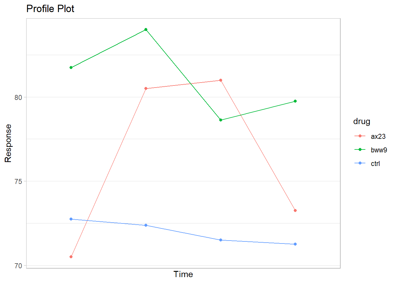

## Fit model
heart_mod <- lm(cbind(y1, y2, y3, y4) ~ drug, data = heart)
man_fit <- car::Anova(heart_mod)
summary(man_fit)
#> 
#> Type II MANOVA Tests:
#> 
#> Sum of squares and products for error:
#>        y1      y2      y3     y4
#> y1 641.00 601.750 535.250 426.00
#> y2 601.75 823.875 615.500 534.25
#> y3 535.25 615.500 655.875 555.25
#> y4 426.00 534.250 555.250 674.50
#> 
#> ------------------------------------------
#>  
#> Term: drug 
#> 
#> Sum of squares and products for the hypothesis:
#>        y1       y2       y3    y4
#> y1 567.00 335.2500  42.7500 387.0
#> y2 335.25 569.0833 404.5417 367.5
#> y3  42.75 404.5417 391.0833 171.0
#> y4 387.00 367.5000 171.0000 316.0
#> 
#> Multivariate Tests: drug
#>                  Df test stat  approx F num Df den Df     Pr(>F)    
#> Pillai            2  1.283456  8.508082      8     38 1.5010e-06 ***
#> Wilks             2  0.079007 11.509581      8     36 6.3081e-08 ***
#> Hotelling-Lawley  2  7.069384 15.022441      8     34 3.9048e-09 ***
#> Roy               2  6.346509 30.145916      4     19 5.4493e-08 ***
#> ---
#> Signif. codes:  0 '***' 0.001 '**' 0.01 '*' 0.05 '.' 0.1 ' ' 1

reject the null hypothesis of no difference in means between treatments

## Contrasts
heart$drug <- factor(heart$drug)
L <- matrix(c(0, 2,
              1, -1,-1, -1), nrow = 3, byrow = T)
colnames(L) <- c("bww9:ctrl", "ax23:rest")
rownames(L) <- unique(heart$drug)
contrasts(heart$drug) <- L
contrasts(heart$drug)
#>      bww9:ctrl ax23:rest
#> ax23         0         2
#> bww9         1        -1
#> ctrl        -1        -1

# do not set contrast L if you do further analysis (e.g., Anova, lm)
# do M matrix instead

M <- matrix(c(1, -1, 0, 0,
              0, 1, -1, 0,
              0, 0, 1, -1), nrow = 4)
## update model to test contrasts
heart_mod2 <- update(heart_mod)
coef(heart_mod2)
#>                  y1         y2        y3    y4
#> (Intercept)   75.00 78.9583333 77.041667 74.75
#> drugbww9:ctrl  4.50  5.8125000  3.562500  4.25
#> drugax23:rest -2.25  0.7708333  1.979167 -0.75

# Hypothesis test for bww9 vs control after transformation M
# same as linearHypothesis(heart_mod, hypothesis.matrix = c(0,1,-1), P = M)
bww9vctrl <-
    car::linearHypothesis(heart_mod2,
                     hypothesis.matrix = c(0, 1, 0),
                     P = M)
bww9vctrl
#> 
#>  Response transformation matrix:
#>    [,1] [,2] [,3]
#> y1    1    0    0
#> y2   -1    1    0
#> y3    0   -1    1
#> y4    0    0   -1
#> 
#> Sum of squares and products for the hypothesis:
#>          [,1]   [,2]     [,3]
#> [1,]  27.5625 -47.25  14.4375
#> [2,] -47.2500  81.00 -24.7500
#> [3,]  14.4375 -24.75   7.5625
#> 
#> Sum of squares and products for error:
#>          [,1]     [,2]    [,3]
#> [1,]  261.375 -141.875  28.000
#> [2,] -141.875  248.750 -19.375
#> [3,]   28.000  -19.375 219.875
#> 
#> Multivariate Tests: 
#>                  Df test stat approx F num Df den Df Pr(>F)
#> Pillai            1 0.2564306 2.184141      3     19 0.1233
#> Wilks             1 0.7435694 2.184141      3     19 0.1233
#> Hotelling-Lawley  1 0.3448644 2.184141      3     19 0.1233
#> Roy               1 0.3448644 2.184141      3     19 0.1233

bww9vctrl <-
    car::linearHypothesis(heart_mod,
                     hypothesis.matrix = c(0, 1, -1),
                     P = M)
bww9vctrl
#> 
#>  Response transformation matrix:
#>    [,1] [,2] [,3]
#> y1    1    0    0
#> y2   -1    1    0
#> y3    0   -1    1
#> y4    0    0   -1
#> 
#> Sum of squares and products for the hypothesis:
#>          [,1]   [,2]     [,3]
#> [1,]  27.5625 -47.25  14.4375
#> [2,] -47.2500  81.00 -24.7500
#> [3,]  14.4375 -24.75   7.5625
#> 
#> Sum of squares and products for error:
#>          [,1]     [,2]    [,3]
#> [1,]  261.375 -141.875  28.000
#> [2,] -141.875  248.750 -19.375
#> [3,]   28.000  -19.375 219.875
#> 
#> Multivariate Tests: 
#>                  Df test stat approx F num Df den Df Pr(>F)
#> Pillai            1 0.2564306 2.184141      3     19 0.1233
#> Wilks             1 0.7435694 2.184141      3     19 0.1233
#> Hotelling-Lawley  1 0.3448644 2.184141      3     19 0.1233
#> Roy               1 0.3448644 2.184141      3     19 0.1233

there is no significant difference in means between the control and bww9 drug

# Hypothesis test for ax23 vs rest after transformation M
axx23vrest <-
    car::linearHypothesis(heart_mod2,
                     hypothesis.matrix = c(0, 0, 1),
                     P = M)
axx23vrest
#> 
#>  Response transformation matrix:
#>    [,1] [,2] [,3]
#> y1    1    0    0
#> y2   -1    1    0
#> y3    0   -1    1
#> y4    0    0   -1
#> 
#> Sum of squares and products for the hypothesis:
#>           [,1]       [,2]      [,3]
#> [1,]  438.0208  175.20833 -395.7292
#> [2,]  175.2083   70.08333 -158.2917
#> [3,] -395.7292 -158.29167  357.5208
#> 
#> Sum of squares and products for error:
#>          [,1]     [,2]    [,3]
#> [1,]  261.375 -141.875  28.000
#> [2,] -141.875  248.750 -19.375
#> [3,]   28.000  -19.375 219.875
#> 
#> Multivariate Tests: 
#>                  Df test stat approx F num Df den Df     Pr(>F)    
#> Pillai            1  0.855364 37.45483      3     19 3.5484e-08 ***
#> Wilks             1  0.144636 37.45483      3     19 3.5484e-08 ***
#> Hotelling-Lawley  1  5.913921 37.45483      3     19 3.5484e-08 ***
#> Roy               1  5.913921 37.45483      3     19 3.5484e-08 ***
#> ---
#> Signif. codes:  0 '***' 0.001 '**' 0.01 '*' 0.05 '.' 0.1 ' ' 1

axx23vrest <-
    car::linearHypothesis(heart_mod,
                     hypothesis.matrix = c(2, -1, 1),
                     P = M)
axx23vrest
#> 
#>  Response transformation matrix:
#>    [,1] [,2] [,3]
#> y1    1    0    0
#> y2   -1    1    0
#> y3    0   -1    1
#> y4    0    0   -1
#> 
#> Sum of squares and products for the hypothesis:
#>           [,1]       [,2]      [,3]
#> [1,]  402.5208  127.41667 -390.9375
#> [2,]  127.4167   40.33333 -123.7500
#> [3,] -390.9375 -123.75000  379.6875
#> 
#> Sum of squares and products for error:
#>          [,1]     [,2]    [,3]
#> [1,]  261.375 -141.875  28.000
#> [2,] -141.875  248.750 -19.375
#> [3,]   28.000  -19.375 219.875
#> 
#> Multivariate Tests: 
#>                  Df test stat approx F num Df den Df     Pr(>F)    
#> Pillai            1  0.842450 33.86563      3     19 7.9422e-08 ***
#> Wilks             1  0.157550 33.86563      3     19 7.9422e-08 ***
#> Hotelling-Lawley  1  5.347205 33.86563      3     19 7.9422e-08 ***
#> Roy               1  5.347205 33.86563      3     19 7.9422e-08 ***
#> ---
#> Signif. codes:  0 '***' 0.001 '**' 0.01 '*' 0.05 '.' 0.1 ' ' 1

there is a significant difference in means between ax23 drug treatment and the rest of the treatments

22.1.2 Profile Analysis

Examine similarities between the treatment effects (between subjects), which is useful for longitudinal analysis. Null is that all treatments have the same average effect.

\[ H_0: \mu_1 = \mu_2 = \dots = \mu_h \]

Equivalently,

\[ H_0: \tau_1 = \tau_2 = \dots = \tau_h \]

The exact nature of the similarities and differences between the treatments can be examined under this analysis.

Sequential steps in profile analysis:

1. Are the profiles parallel? (i.e., is there no interaction between treatment and time)
2. Are the profiles coincidental? (i.e., are the profiles identical?)
3. Are the profiles horizontal? (i.e., are there no differences between any time points?)

If we reject the null hypothesis that the profiles are parallel, we can test

• Are there differences among groups within some subset of the total time points?

• Are there differences among time points in a particular group (or groups)?

• Are there differences within some subset of the total time points in a particular group (or groups)?

Example

• 4 times (p = 4)

• 3 treatments (h=3)

22.1.2.1 Parallel Profile

Are the profiles for each population identical expect for a mean shift?

\[ \begin{aligned} H_0: \mu_{11} - \mu_{21} - \mu_{12} - \mu_{22} = &\dots = \mu_{1t} - \mu_{2t} \\ \mu_{11} - \mu_{31} - \mu_{12} - \mu_{32} = &\dots = \mu_{1t} - \mu_{3t} \\ &\dots \end{aligned} \]

for \(h-1\) equations

Equivalently,

\[ H_0: \mathbf{LBM = 0} \]

\[ \mathbf{LBM} = \left[ \begin{array} {ccc} 1 & -1 & 0 \\ 1 & 0 & -1 \end{array} \right] \left[ \begin{array} {ccc} \mu_{11} & \dots & \mu_{14} \\ \mu_{21} & \dots & \mu_{24} \\ \mu_{31} & \dots & \mu_{34} \end{array} \right] \left[ \begin{array} {ccc} 1 & 1 & 1 \\ -1 & 0 & 0 \\ 0 & -1 & 0 \\ 0 & 0 & -1 \end{array} \right] = \mathbf{0} \]

where this is the cell means parameterization of \(\mathbf{B}\)

The multiplication of the first 2 matrices \(\mathbf{LB}\) is

\[ \left[ \begin{array} {cccc} \mu_{11} - \mu_{21} & \mu_{12} - \mu_{22} & \mu_{13} - \mu_{23} & \mu_{14} - \mu_{24}\\ \mu_{11} - \mu_{31} & \mu_{12} - \mu_{32} & \mu_{13} - \mu_{33} & \mu_{14} - \mu_{34} \end{array} \right] \]

which is the differences in treatment means at the same time

Multiplying by \(\mathbf{M}\), we get the comparison across time

\[ \left[ \begin{array} {ccc} (\mu_{11} - \mu_{21}) - (\mu_{12} - \mu_{22}) & (\mu_{11} - \mu_{21}) -(\mu_{13} - \mu_{23}) & (\mu_{11} - \mu_{21}) - (\mu_{14} - \mu_{24}) \\ (\mu_{11} - \mu_{31}) - (\mu_{12} - \mu_{32}) & (\mu_{11} - \mu_{31}) - (\mu_{13} - \mu_{33}) & (\mu_{11} - \mu_{31}) -(\mu_{14} - \mu_{34}) \end{array} \right] \]

Alternatively, we can also use the effects parameterization

\[ \mathbf{LBM} = \left[ \begin{array} {cccc} 0 & 1 & -1 & 0 \\ 0 & 1 & 0 & -1 \end{array} \right] \left[ \begin{array} {c} \mu' \\ \tau'_1 \\ \tau_2' \\ \tau_3' \end{array} \right] \left[ \begin{array} {ccc} 1 & 1 & 1 \\ -1 & 0 & 0 \\ 0 & -1 & 0 \\ 0 & 0 & -1 \end{array} \right] = \mathbf{0} \]

In both parameterizations, \(rank(\mathbf{L}) = h-1\) and \(rank(\mathbf{M}) = p-1\)

We could also choose \(\mathbf{L}\) and \(\mathbf{M}\) in other forms

\[ \mathbf{L} = \left[ \begin{array} {cccc} 0 & 1 & 0 & -1 \\ 0 & 0 & 1 & -1 \end{array} \right] \]

and

\[ \mathbf{M} = \left[ \begin{array} {ccc} 1 & 0 & 0 \\ -1 & 1 & 0 \\ 0 & -1 & 1 \\ 0 & 0 & -1 \end{array} \right] \]

and still obtain the same result.

22.1.2.2 Coincidental Profiles

After we have evidence that the profiles are parallel (i.e., fail to reject the parallel profile test), we can ask whether they are identical?

Given profiles are parallel, then if the sums of the components of \(\mu_i\) are identical for all the treatments, then the profiles are identical.

\[ H_0: \mathbf{1'}_p \mu_1 = \mathbf{1'}_p \mu_2 = \dots = \mathbf{1'}_p \mu_h \]

Equivalently,

\[ H_0: \mathbf{LBM} = \mathbf{0} \]

where for the cell means parameterization

\[ \mathbf{L} = \left[ \begin{array} {ccc} 1 & 0 & -1 \\ 0 & 1 & -1 \end{array} \right] \]

and

\[ \mathbf{M} = \left[ \begin{array} {cccc} 1 & 1 & 1 & 1 \end{array} \right]' \]

multiplication yields

\[ \left[ \begin{array} {c} (\mu_{11} + \mu_{12} + \mu_{13} + \mu_{14}) - (\mu_{31} + \mu_{32} + \mu_{33} + \mu_{34}) \\ (\mu_{21} + \mu_{22} + \mu_{23} + \mu_{24}) - (\mu_{31} + \mu_{32} + \mu_{33} + \mu_{34}) \end{array} \right] = \left[ \begin{array} {c} 0 \\ 0 \end{array} \right] \]

Different choices of \(\mathbf{L}\) and \(\mathbf{M}\) can yield the same result

22.1.2.3 Horizontal Profiles

Given that we can’t reject the null hypothesis that all \(h\) profiles are the same, we can ask whether all of the elements of the common profile equal? (i.e., horizontal)

\[ H_0: \mathbf{LBM} = \mathbf{0} \]

\[ \mathbf{L} = \left[ \begin{array} {ccc} 1 & 0 & 0 \end{array} \right] \]

and

\[ \mathbf{M} = \left[ \begin{array} {ccc} 1 & 0 & 0 \\ -1 & 1 & 0 \\ 0 & -1 & 1 \\ 0 & 0 & -1 \end{array} \right] \]

hence,

\[ \left[ \begin{array} {ccc} (\mu_{11} - \mu_{12}) & (\mu_{12} - \mu_{13}) & (\mu_{13} + \mu_{14}) \end{array} \right] = \left[ \begin{array} {ccc} 0 & 0 & 0 \end{array} \right] \]

Note:

• If we fail to reject all 3 hypotheses, then we fail to reject the null hypotheses of both no difference between treatments and no differences between traits.

Test	Equivalent test for
Parallel profile	Interaction
Coincidental profile	main effect of between-subjects factor
Horizontal profile	main effect of repeated measures factor

profile_fit <-
    pbg(
        data = as.matrix(heart[, 2:5]),
        group = as.matrix(heart[, 1]),
        original.names = TRUE,
        profile.plot = FALSE
    )
summary(profile_fit)
#> Call:
#> pbg(data = as.matrix(heart[, 2:5]), group = as.matrix(heart[, 
#>     1]), original.names = TRUE, profile.plot = FALSE)
#> 
#> Hypothesis Tests:
#> $`Ho: Profiles are parallel`
#>   Multivariate.Test Statistic  Approx.F num.df den.df      p.value
#> 1             Wilks 0.1102861 12.737599      6     38 7.891497e-08
#> 2            Pillai 1.0891707  7.972007      6     40 1.092397e-05
#> 3  Hotelling-Lawley 6.2587852 18.776356      6     36 9.258571e-10
#> 4               Roy 5.9550887 39.700592      3     20 1.302458e-08
#> 
#> $`Ho: Profiles have equal levels`
#>             Df Sum Sq Mean Sq F value  Pr(>F)   
#> group        2  328.7  164.35   5.918 0.00915 **
#> Residuals   21  583.2   27.77                   
#> ---
#> Signif. codes:  0 '***' 0.001 '**' 0.01 '*' 0.05 '.' 0.1 ' ' 1
#> 
#> $`Ho: Profiles are flat`
#>          F df1 df2      p-value
#> 1 14.30928   3  19 4.096803e-05
# reject null hypothesis of parallel profiles
# reject the null hypothesis of coincidental profiles
# reject the null hypothesis that the profiles are flat

22.1.3 Summary

22.2 Principal Components

• Unsupervised learning
• find important features
• reduce the dimensions of the data set
• “decorrelate” multivariate vectors that have dependence.
• uses eigenvector/eigvenvalue decomposition of covariance (correlation) matrices.

According to the “spectral decomposition theorem”, if \(\mathbf{\Sigma}_{p \times p}\) i s a positive semi-definite, symmetric, real matrix, then there exists an orthogonal matrix \(\mathbf{A}\) such that \(\mathbf{A'\Sigma A} = \Lambda\) where \(\Lambda\) is a diagonal matrix containing the eigenvalues \(\mathbf{\Sigma}\)

\[ \mathbf{\Lambda} = \left( \begin{array} {cccc} \lambda_1 & 0 & \ldots & 0 \\ 0 & \lambda_2 & \ldots & 0 \\ \vdots & \vdots & \ddots & \vdots \\ 0 & 0 & \ldots & \lambda_p \end{array} \right) \]

\[ \mathbf{A} = \left( \begin{array} {cccc} \mathbf{a}_1 & \mathbf{a}_2 & \ldots & \mathbf{a}_p \end{array} \right) \]

the i-th column of \(\mathbf{A}\) , \(\mathbf{a}_i\), is the i-th \(p \times 1\) eigenvector of \(\mathbf{\Sigma}\) that corresponds to the eigenvalue, \(\lambda_i\) , where \(\lambda_1 \ge \lambda_2 \ge \ldots \ge \lambda_p\) . Alternatively, express in matrix decomposition:

\[ \mathbf{\Sigma} = \mathbf{A \Lambda A}' \]

\[ \mathbf{\Sigma} = \mathbf{A} \left( \begin{array} {cccc} \lambda_1 & 0 & \ldots & 0 \\ 0 & \lambda_2 & \ldots & 0 \\ \vdots & \vdots& \ddots & \vdots \\ 0 & 0 & \ldots & \lambda_p \end{array} \right) \mathbf{A}' = \sum_{i=1}^p \lambda_i \mathbf{a}_i \mathbf{a}_i' \]

where the outer product \(\mathbf{a}_i \mathbf{a}_i'\) is a \(p \times p\) matrix of rank 1.

For example,

\(\mathbf{x} \sim N_2(\mathbf{\mu}, \mathbf{\Sigma})\)

\[ \mathbf{\mu} = \left( \begin{array} {c} 5 \\ 12 \end{array} \right); \mathbf{\Sigma} = \left( \begin{array} {cc} 4 & 1 \\ 1 & 2 \end{array} \right) \]

library(MASS)
mu = as.matrix(c(5, 12))
Sigma = matrix(c(4, 1, 1, 2), nrow = 2, byrow = T)
sim <- mvrnorm(n = 1000, mu = mu, Sigma = Sigma)
plot(sim[, 1], sim[, 2])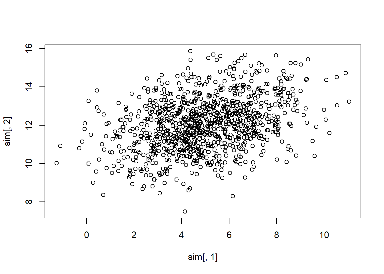

Here,

\[ \mathbf{A} = \left( \begin{array} {cc} 0.9239 & -0.3827 \\ 0.3827 & 0.9239 \\ \end{array} \right) \]

Columns of \(\mathbf{A}\) are the eigenvectors for the decomposition

Under matrix multiplication (\(\mathbf{A'\Sigma A}\) or \(\mathbf{A'A}\) ), the off-diagonal elements equal to 0

Multiplying data by this matrix (i.e., projecting the data onto the orthogonal axes); the distribution of the resulting data (i.e., “scores”) is

\[ N_2 (\mathbf{A'\mu,A'\Sigma A}) = N_2 (\mathbf{A'\mu, \Lambda}) \]

Equivalently,

\[ \mathbf{y} = \mathbf{A'x} \sim N \left[ \left( \begin{array} {c} 9.2119 \\ 9.1733 \end{array} \right), \left( \begin{array} {cc} 4.4144 & 0 \\ 0 & 1.5859 \end{array} \right) \right] \]

A_matrix = matrix(c(0.9239, -0.3827, 0.3827, 0.9239),
                  nrow = 2,
                  byrow = T)
t(A_matrix) %*% A_matrix
#>          [,1]     [,2]
#> [1,] 1.000051 0.000000
#> [2,] 0.000000 1.000051

sim1 <-
    mvrnorm(
        n = 1000,
        mu = t(A_matrix) %*% mu,
        Sigma = t(A_matrix) %*% Sigma %*% A_matrix
    )
plot(sim1[, 1], sim1[, 2])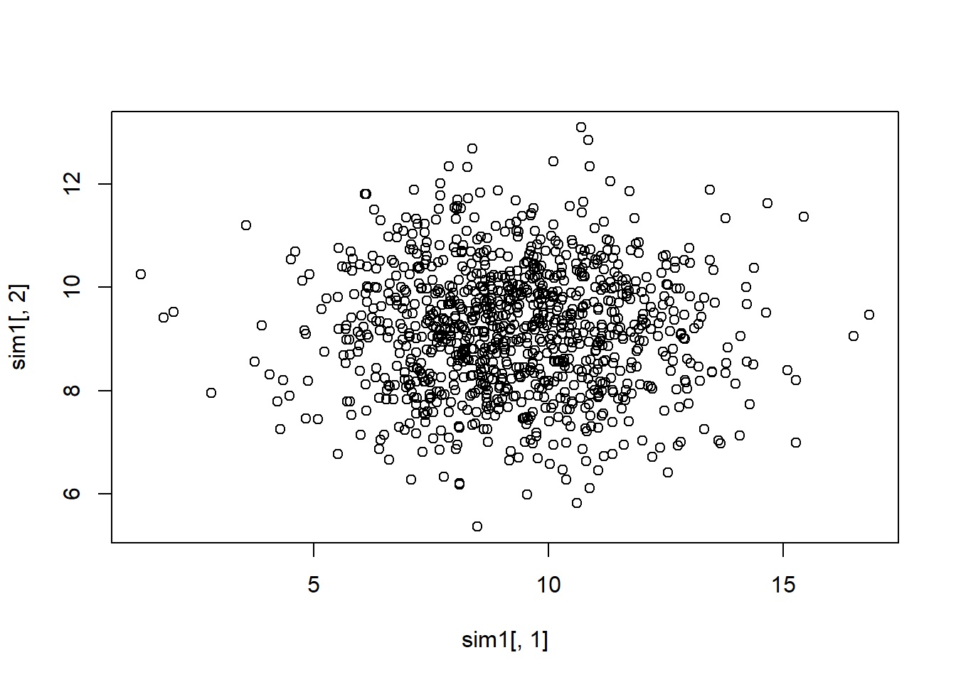

No more dependence in the data structure, plot

Notes:

• The i-th eigenvalue is the variance of a linear combination of the elements of \(\mathbf{x}\) ; \(var(y_i) = var(\mathbf{a'_i x}) = \lambda_i\)

• The values on the transformed set of axes (i.e., the \(y_i\)’s) are called the scores. These are the orthogonal projections of the data onto the “new principal component axes

• Variances of \(y_1\) are greater than those for any other possible projection

Covariance matrix decomposition and projection onto orthogonal axes = PCA

22.2.1 Population Principal Components

\(p \times 1\) vectors \(\mathbf{x}_1, \dots , \mathbf{x}_n\) which are iid with \(var(\mathbf{x}_i) = \mathbf{\Sigma}\)

• The first PC is the linear combination \(y_1 = \mathbf{a}_1' \mathbf{x} = a_{11}x_1 + \dots + a_{1p}x_p\) with \(\mathbf{a}_1' \mathbf{a}_1 = 1\) such that \(var(y_1)\) is the maximum of all linear combinations of \(\mathbf{x}\) which have unit length

• The second PC is the linear combination \(y_1 = \mathbf{a}_2' \mathbf{x} = a_{21}x_1 + \dots + a_{2p}x_p\) with \(\mathbf{a}_2' \mathbf{a}_2 = 1\) such that \(var(y_1)\) is the maximum of all linear combinations of \(\mathbf{x}\) which have unit length and uncorrelated with \(y_1\) (i.e., \(cov(\mathbf{a}_1' \mathbf{x}, \mathbf{a}'_2 \mathbf{x}) =0\)

• continues for all \(y_i\) to \(y_p\)

\(\mathbf{a}_i\)’s are those that make up the matrix \(\mathbf{A}\) in the symmetric decomposition \(\mathbf{A'\Sigma A} = \mathbf{\Lambda}\) , where \(var(y_1) = \lambda_1, \dots , var(y_p) = \lambda_p\) And the total variance of \(\mathbf{x}\) is

\[ \begin{aligned} var(x_1) + \dots + var(x_p) &= tr(\Sigma) = \lambda_1 + \dots + \lambda_p \\ &= var(y_1) + \dots + var(y_p) \end{aligned} \]

Data Reduction

To reduce the dimension of data from p (original) to k dimensions without much “loss of information”, we can use properties of the population principal components

• Suppose \(\mathbf{\Sigma} \approx \sum_{i=1}^k \lambda_i \mathbf{a}_i \mathbf{a}_i'\) . Even thought the true variance-covariance matrix has rank \(p\) , it can be be well approximate by a matrix of rank k (k <p)

• New “traits” are linear combinations of the measured traits. We can attempt to make meaningful interpretation fo the combinations (with orthogonality constraints).

• The proportion of the total variance accounted for by the j-th principal component is

\[ \frac{var(y_j)}{\sum_{i=1}^p var(y_i)} = \frac{\lambda_j}{\sum_{i=1}^p \lambda_i} \]

• The proportion of the total variation accounted for by the first k principal components is \(\frac{\sum_{i=1}^k \lambda_i}{\sum_{i=1}^p \lambda_i}\)

• Above example , we have \(4.4144/(4+2) = .735\) of the total variability can be explained by the first principal component

22.2.2 Sample Principal Components

Since \(\mathbf{\Sigma}\) is unknown, we use

\[ \mathbf{S} = \frac{1}{n-1}\sum_{i=1}^n (\mathbf{x}_i - \bar{\mathbf{x}})(\mathbf{x}_i - \bar{\mathbf{x}})' \]

Let \(\hat{\lambda}_1 \ge \hat{\lambda}_2 \ge \dots \ge \hat{\lambda}_p \ge 0\) be the eigenvalues of \(\mathbf{S}\) and \(\hat{\mathbf{a}}_1, \hat{\mathbf{a}}_2, \dots, \hat{\mathbf{a}}_p\) denote the eigenvectors of \(\mathbf{S}\)

Then, the i-th sample principal component score (or principal component or score) is

\[ \hat{y}_{ij} = \sum_{k=1}^p \hat{a}_{ik}x_{kj} = \hat{\mathbf{a}}_i'\mathbf{x}_j \]

Properties of Sample Principal Components

• The estimated variance of \(y_i = \hat{\mathbf{a}}_i'\mathbf{x}_j\) is \(\hat{\lambda}_i\)

• The sample covariance between \(\hat{y}_i\) and \(\hat{y}_{i'}\) is 0 when \(i \neq i'\)

• The proportion of the total sample variance accounted for by the i-th sample principal component is \(\frac{\hat{\lambda}_i}{\sum_{k=1}^p \hat{\lambda}_k}\)

• The estimated correlation between the \(i\)-th principal component score and the \(l\)-th attribute of \(\mathbf{x}\) is

\[ r_{x_l , \hat{y}_i} = \frac{\hat{a}_{il}\sqrt{\lambda_i}}{\sqrt{s_{ll}}} \]

• The correlation coefficient is typically used to interpret the components (i.e., if this correlation is high then it suggests that the l-th original trait is important in the i-th principle component). According to R. A. Johnson, Wichern, et al. (2002), pp.433-434, \(r_{x_l, \hat{y}_i}\) only measures the univariate contribution of an individual X to a component Y without taking into account the presence of the other X’s. Hence, some prefer \(\hat{a}_{il}\) coefficient to interpret the principal component.

• \(r_{x_l, \hat{y}_i} ; \hat{a}_{il}\) are referred to as “loadings”

To use k principal components, we must calculate the scores for each data vector in the sample

\[ \mathbf{y}_j = \left( \begin{array} {c} y_{1j} \\ y_{2j} \\ \vdots \\ y_{kj} \end{array} \right) = \left( \begin{array} {c} \hat{\mathbf{a}}_1' \mathbf{x}_j \\ \hat{\mathbf{a}}_2' \mathbf{x}_j \\ \vdots \\ \hat{\mathbf{a}}_k' \mathbf{x}_j \end{array} \right) = \left( \begin{array} {c} \hat{\mathbf{a}}_1' \\ \hat{\mathbf{a}}_2' \\ \vdots \\ \hat{\mathbf{a}}_k' \end{array} \right) \mathbf{x}_j \]

Issues:

• Large sample theory exists for eigenvalues and eigenvectors of sample covariance matrices if inference is necessary. But we do not do inference with PCA, we only use it as exploratory or descriptive analysis.

• PC is not invariant to changes in scale (Exception: if all trait are rescaled by multiplying by the same constant, such as feet to inches).

  • PCA based on the correlation matrix \(\mathbf{R}\) is different than that based on the covariance matrix \(\mathbf{\Sigma}\)

  • PCA for the correlation matrix is just rescaling each trait to have unit variance

  • Transform \(\mathbf{x}\) to \(\mathbf{z}\) where \(z_{ij} = (x_{ij} - \bar{x}_i)/\sqrt{s_{ii}}\) where the denominator affects the PCA

  • After transformation, \(cov(\mathbf{z}) = \mathbf{R}\)

  • PCA on \(\mathbf{R}\) is calculated in the same way as that on \(\mathbf{S}\) (where \(\hat{\lambda}{}_1 + \dots + \hat{\lambda}{}_p = p\) )

  • The use of \(\mathbf{R}, \mathbf{S}\) depends on the purpose of PCA.

    • If the scale of the observations if different, covariance matrix is more preferable. but if they are dramatically different, analysis can still be dominated by the large variance traits.

  • How many PCs to use can be guided by

    • Scree Graphs: plot the eigenvalues against their indices. Look for the “elbow” where the steep decline in the graph suddenly flattens out; or big gaps.

    • minimum Percent of total variation (e.g., choose enough components to have 50% or 90%). can be used for interpretations.

    • Kaiser’s rule: use only those PC with eigenvalues larger than 1 (applied to PCA on the correlation matrix) - ad hoc

    • Compare to the eigenvalue scree plot of data to the scree plot when the data are randomized.

22.2.3 Application

PCA on the covariance matrix is usually not preferred due to the fact that PCA is not invariant to changes in scale. Hence, PCA on the correlation matrix is more preferred

This also addresses the problem of multicollinearity

The eigvenvectors may differ by a multiplication of -1 for different implementation, but same interpretation.

library(tidyverse)
## Read in and check data
stock <- read.table("images/stock.dat")
names(stock) <- c("allied", "dupont", "carbide", "exxon", "texaco")
str(stock)
#> 'data.frame':    100 obs. of  5 variables:
#>  $ allied : num  0 0.027 0.1228 0.057 0.0637 ...
#>  $ dupont : num  0 -0.04485 0.06077 0.02995 -0.00379 ...
#>  $ carbide: num  0 -0.00303 0.08815 0.06681 -0.03979 ...
#>  $ exxon  : num  0.0395 -0.0145 0.0862 0.0135 -0.0186 ...
#>  $ texaco : num  0 0.0435 0.0781 0.0195 -0.0242 ...

## Covariance matrix of data
cov(stock)
#>               allied       dupont      carbide        exxon       texaco
#> allied  0.0016299269 0.0008166676 0.0008100713 0.0004422405 0.0005139715
#> dupont  0.0008166676 0.0012293759 0.0008276330 0.0003868550 0.0003109431
#> carbide 0.0008100713 0.0008276330 0.0015560763 0.0004872816 0.0004624767
#> exxon   0.0004422405 0.0003868550 0.0004872816 0.0008023323 0.0004084734
#> texaco  0.0005139715 0.0003109431 0.0004624767 0.0004084734 0.0007587370

## Correlation matrix of data
cor(stock)
#>            allied    dupont   carbide     exxon    texaco
#> allied  1.0000000 0.5769244 0.5086555 0.3867206 0.4621781
#> dupont  0.5769244 1.0000000 0.5983841 0.3895191 0.3219534
#> carbide 0.5086555 0.5983841 1.0000000 0.4361014 0.4256266
#> exxon   0.3867206 0.3895191 0.4361014 1.0000000 0.5235293
#> texaco  0.4621781 0.3219534 0.4256266 0.5235293 1.0000000

# cov(scale(stock)) # give the same result

## PCA with covariance
cov_pca <- prcomp(stock) 
# uses singular value decomposition for calculation and an N -1 divisor
# alternatively, princomp can do PCA via spectral decomposition, 
# but it has worse numerical accuracy

# eigen values
cov_results <- data.frame(eigen_values = cov_pca$sdev ^ 2)
cov_results %>%
    mutate(proportion = eigen_values / sum(eigen_values),
           cumulative = cumsum(proportion)) 
#>   eigen_values proportion cumulative
#> 1 0.0035953867 0.60159252  0.6015925
#> 2 0.0007921798 0.13255027  0.7341428
#> 3 0.0007364426 0.12322412  0.8573669
#> 4 0.0005086686 0.08511218  0.9424791
#> 5 0.0003437707 0.05752091  1.0000000
# first 2 PCs account for 73% variance in the data

# eigen vectors
cov_pca$rotation # prcomp calls rotation
#>               PC1         PC2        PC3         PC4         PC5
#> allied  0.5605914  0.73884565 -0.1260222  0.28373183 -0.20846832
#> dupont  0.4698673 -0.09286987 -0.4675066 -0.68793190  0.28069055
#> carbide 0.5473322 -0.65401929 -0.1140581  0.50045312 -0.09603973
#> exxon   0.2908932 -0.11267353  0.6099196 -0.43808002 -0.58203935
#> texaco  0.2842017  0.07103332  0.6168831  0.06227778  0.72784638
# princomp calls loadings.

# first PC = overall average
# second PC compares Allied to Carbide

## PCA with correlation
#same as scale(stock) %>% prcomp
cor_pca <- prcomp(stock, scale = T)



# eigen values
cor_results <- data.frame(eigen_values = cor_pca$sdev ^ 2)
cor_results %>%
    mutate(proportion = eigen_values / sum(eigen_values),
           cumulative = cumsum(proportion))
#>   eigen_values proportion cumulative
#> 1    2.8564869 0.57129738  0.5712974
#> 2    0.8091185 0.16182370  0.7331211
#> 3    0.5400440 0.10800880  0.8411299
#> 4    0.4513468 0.09026936  0.9313992
#> 5    0.3430038 0.06860076  1.0000000

# first egiven values corresponds to less variance 
# than PCA based on the covariance matrix

# eigen vectors
cor_pca$rotation
#>               PC1        PC2        PC3        PC4        PC5
#> allied  0.4635405 -0.2408499  0.6133570 -0.3813727  0.4532876
#> dupont  0.4570764 -0.5090997 -0.1778996 -0.2113068 -0.6749814
#> carbide 0.4699804 -0.2605774 -0.3370355  0.6640985  0.3957247
#> exxon   0.4216770  0.5252647 -0.5390181 -0.4728036  0.1794482
#> texaco  0.4213291  0.5822416  0.4336029  0.3812273 -0.3874672
# interpretation of PC2 is different from above: 
# it is a comparison of Allied, Dupont and Carbid to Exxon and Texaco 

Covid Example

To reduce collinearity problem in this dataset, we can use principal components as regressors.

load('images/MOcovid.RData')
covidpca <- prcomp(ndat[,-1],scale = T,center = T)

covidpca$rotation[,1:2]
#>                                                          PC1         PC2
#> X..Population.in.Rural.Areas                      0.32865838  0.05090955
#> Area..sq..miles.                                  0.12014444 -0.28579183
#> Population.density..sq..miles.                   -0.29670124  0.28312922
#> Literacy.rate                                    -0.12517700 -0.08999542
#> Families                                         -0.25856941  0.16485752
#> Area.of.farm.land..sq..miles.                     0.02101106 -0.31070363
#> Number.of.farms                                  -0.03814582 -0.44809679
#> Average.value.of.all.property.per.farm..dollars. -0.05410709  0.14404306
#> Estimation.of.rurality..                         -0.19040210  0.12089501
#> Male..                                            0.02182394 -0.09568768
#> Number.of.Physcians.per.100.000                  -0.31451606  0.13598026
#> average.age                                       0.29414708  0.35593459
#> X0.4.age.proportion                              -0.11431336 -0.23574057
#> X20.44.age.proportion                            -0.32802128 -0.22718550
#> X65.and.over.age.proportion                       0.30585033  0.32201626
#> prop..White..nonHisp                              0.35627561 -0.14142646
#> prop..Hispanic                                   -0.16655381 -0.15105342
#> prop..Black                                      -0.33333359  0.24405802


# Variability of each principal component: pr.var
pr.var <- covidpca$sdev ^ 2
# Variance explained by each principal component: pve
pve <- pr.var / sum(pr.var)
plot(
    pve,
    xlab = "Principal Component",
    ylab = "Proportion of Variance Explained",
    ylim = c(0, 0.5),
    type = "b"
)

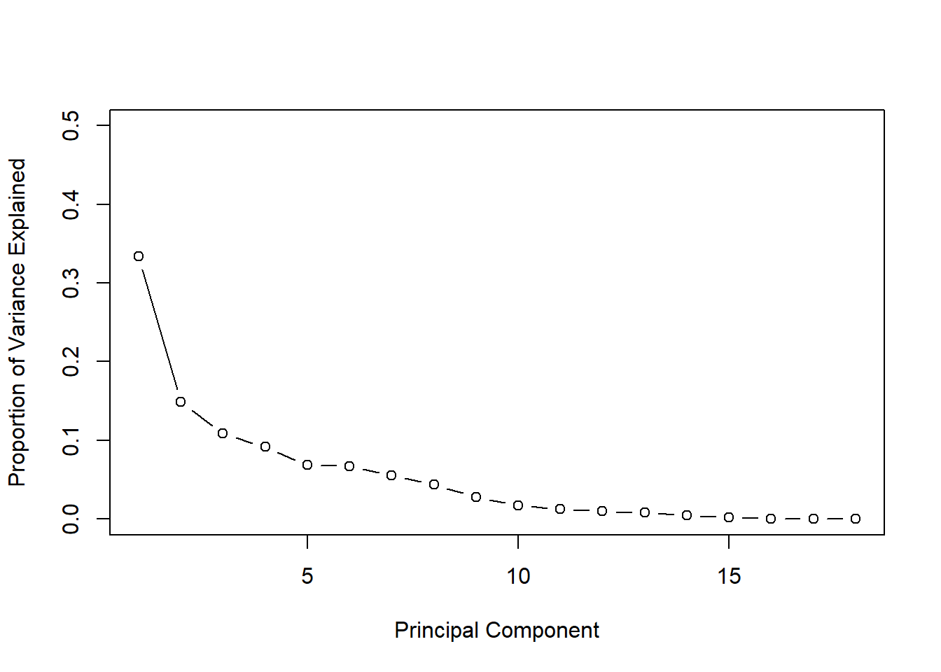
plot(
    cumsum(pve),
    xlab = "Principal Component",
    ylab = "Cumulative Proportion of Variance Explained",
    ylim = c(0, 1),
    type = "b"
)

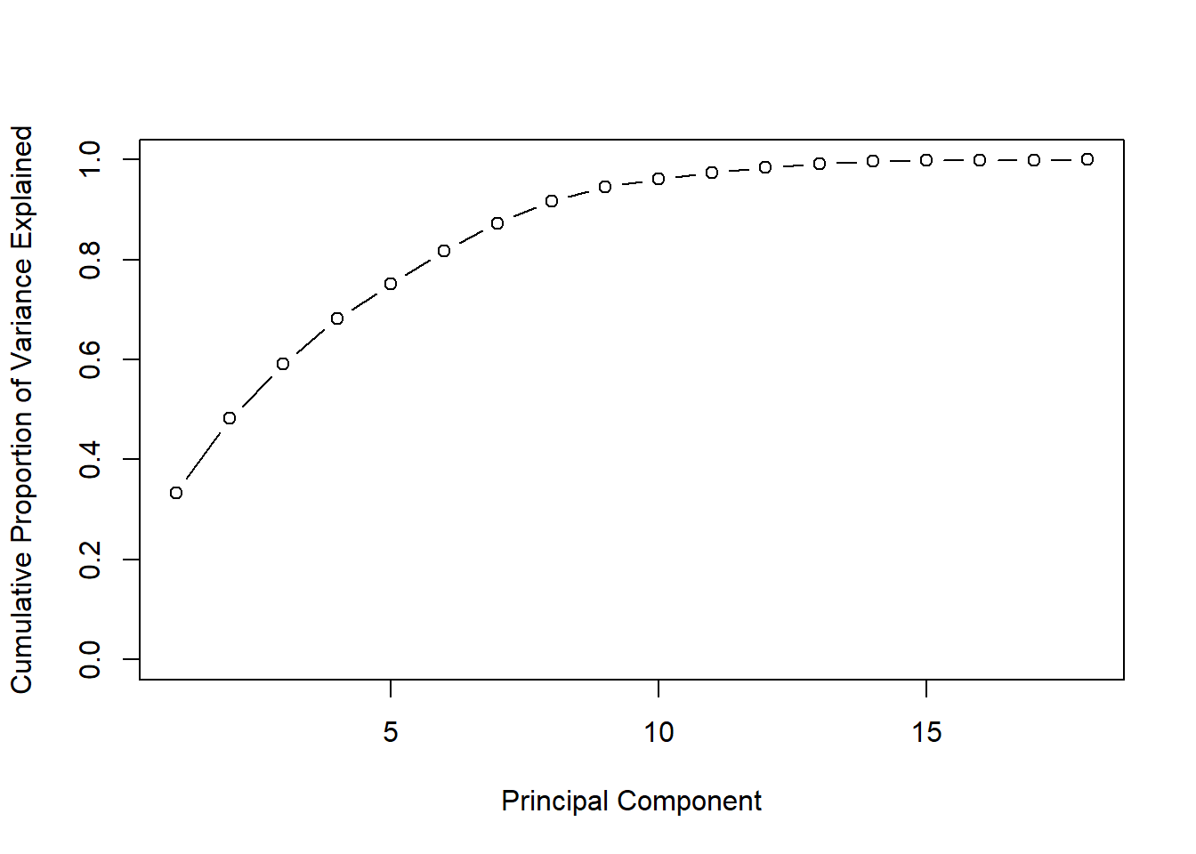
# the first six principe account for around 80% of the variance. 


#using base lm function for PC regression
pcadat <- data.frame(covidpca$x[, 1:6])
pcadat$y <- ndat$Y
pcr.man <- lm(log(y) ~ ., pcadat)
mean(pcr.man$residuals ^ 2)
#> [1] 0.03453371

#comparison to lm w/o prin comps
lm.fit <- lm(log(Y) ~ ., data = ndat)
mean(lm.fit$residuals ^ 2)
#> [1] 0.02335128

MSE for the PC-based model is larger than regular regression, because models with a large degree of collinearity can still perform well.

pcr function in pls can be used for fitting PC regression (it will select the optimal number of components in the model).

22.3 Factor Analysis

Purpose

• Using a few linear combinations of underlying unobservable (latent) traits, we try to describe the covariance relationship among a large number of measured traits

• Similar to PCA, but factor analysis is model based

More details can be found on PSU stat or UMN stat

Let \(\mathbf{y}\) be the set of \(p\) measured variables

\(E(\mathbf{y}) = \mathbf{\mu}\)

\(var(\mathbf{y}) = \mathbf{\Sigma}\)

We have

\[ \begin{aligned} \mathbf{y} - \mathbf{\mu} &= \mathbf{Lf} + \epsilon \\ &= \left( \begin{array} {c} l_{11}f_1 + l_{12}f_2 + \dots + l_{tm}f_m \\ \vdots \\ l_{p1}f_1 + l_{p2}f_2 + \dots + l_{pm} f_m \end{array} \right) + \left( \begin{array} {c} \epsilon_1 \\ \vdots \\ \epsilon_p \end{array} \right) \end{aligned} \]

where

• \(\mathbf{y} - \mathbf{\mu}\) = the p centered measurements

• \(\mathbf{L}\) = \(p \times m\) matrix of factor loadings

• \(\mathbf{f}\) = unobserved common factors for the population

• \(\mathbf{\epsilon}\) = random errors (i.e., variation that is not accounted for by the common factors).

We want \(m\) (the number of factors) to be much smaller than \(p\) (the number of measured attributes)

Restrictions on the model

• \(E(\epsilon) = \mathbf{0}\)

• \(var(\epsilon) = \Psi_{p \times p} = diag( \psi_1, \dots, \psi_p)\)

• \(\mathbf{\epsilon}, \mathbf{f}\) are independent

• Additional assumption could be \(E(\mathbf{f}) = \mathbf{0}, var(\mathbf{f}) = \mathbf{I}_{m \times m}\) (known as the orthogonal factor model) , which imposes the following covariance structure on \(\mathbf{y}\)

\[ \begin{aligned} var(\mathbf{y}) = \mathbf{\Sigma} &= var(\mathbf{Lf} + \mathbf{\epsilon}) \\ &= var(\mathbf{Lf}) + var(\epsilon) \\ &= \mathbf{L} var(\mathbf{f}) \mathbf{L}' + \mathbf{\Psi} \\ &= \mathbf{LIL}' + \mathbf{\Psi} \\ &= \mathbf{LL}' + \mathbf{\Psi} \end{aligned} \]

Since \(\mathbf{\Psi}\) is diagonal, the off-diagonal elements of \(\mathbf{LL}'\) are \(\sigma_{ij}\), the co variances in \(\mathbf{\Sigma}\), which means \(cov(y_i, y_j) = \sum_{k=1}^m l_{ik}l_{jk}\) and the covariance of \(\mathbf{y}\) is completely determined by the m factors ( \(m <<p\))

\(var(y_i) = \sum_{k=1}^m l_{ik}^2 + \psi_i\) where \(\psi_i\) is the specific variance and the summation term is the i-th communality (i.e., portion of the variance of the i-th variable contributed by the \(m\) common factors (\(h_i^2 = \sum_{k=1}^m l_{ik}^2\))

The factor model is only uniquely determined up to an orthogonal transformation of the factors.

Let \(\mathbf{T}_{m \times m}\) be an orthogonal matrix \(\mathbf{TT}' = \mathbf{T'T} = \mathbf{I}\) then

\[ \begin{aligned} \mathbf{y} - \mathbf{\mu} &= \mathbf{Lf} + \epsilon \\ &= \mathbf{LTT'f} + \epsilon \\ &= \mathbf{L}^*(\mathbf{T'f}) + \epsilon & \text{where } \mathbf{L}^* = \mathbf{LT} \end{aligned} \]

and

\[ \begin{aligned} \mathbf{\Sigma} &= \mathbf{LL}' + \mathbf{\Psi} \\ &= \mathbf{LTT'L} + \mathbf{\Psi} \\ &= (\mathbf{L}^*)(\mathbf{L}^*)' + \mathbf{\Psi} \end{aligned} \]

Hence, any orthogonal transformation of the factors is an equally good description of the correlations among the observed traits.

Let \(\mathbf{y} = \mathbf{Cx}\) , where \(\mathbf{C}\) is any diagonal matrix, then \(\mathbf{L}_y = \mathbf{CL}_x\) and \(\mathbf{\Psi}_y = \mathbf{C\Psi}_x\mathbf{C}\)

Hence, we can see that factor analysis is also invariant to changes in scale

22.3.1 Methods of Estimation

To estimate \(\mathbf{L}\)

1. Principal Component Method
2. Principal Factor Method
3. 22.3.1.3

22.3.1.1 Principal Component Method

Spectral decomposition

\[ \begin{aligned} \mathbf{\Sigma} &= \lambda_1 \mathbf{a}_1 \mathbf{a}_1' + \dots + \lambda_p \mathbf{a}_p \mathbf{a}_p' \\ &= \mathbf{A\Lambda A}' \\ &= \sum_{k=1}^m \lambda+k \mathbf{a}_k \mathbf{a}_k' + \sum_{k= m+1}^p \lambda_k \mathbf{a}_k \mathbf{a}_k' \\ &= \sum_{k=1}^m l_k l_k' + \sum_{k=m+1}^p \lambda_k \mathbf{a}_k \mathbf{a}_k' \end{aligned} \]

where \(l_k = \mathbf{a}_k \sqrt{\lambda_k}\) and the second term is not diagonal in general.

Assume

\[ \psi_i = \sigma_{ii} - \sum_{k=1}^m l_{ik}^2 = \sigma_{ii} - \sum_{k=1}^m \lambda_i a_{ik}^2 \]

then

\[ \mathbf{\Sigma} \approx \mathbf{LL}' + \mathbf{\Psi} \]

To estimate \(\mathbf{L}\) and \(\Psi\) , we use the expected eigenvalues and eigenvectors from \(\mathbf{S}\) or \(\mathbf{R}\)

• The estimated factor loadings don’t change as the number of actors increases

• The diagonal elements of \(\hat{\mathbf{L}}\hat{\mathbf{L}}' + \hat{\mathbf{\Psi}}\) are equal to the diagonal elements of \(\mathbf{S}\) and \(\mathbf{R}\), but the covariances may not be exactly reproduced

• We select \(m\) so that the off-diagonal elements close to the values in \(\mathbf{S}\) (or to make the off-diagonal elements of \(\mathbf{S} - \hat{\mathbf{L}} \hat{\mathbf{L}}' + \hat{\mathbf{\Psi}}\) small)

22.3.1.2 Principal Factor Method

Consider modeling the correlation matrix, \(\mathbf{R} = \mathbf{L} \mathbf{L}' + \mathbf{\Psi}\) . Then

\[ \mathbf{L} \mathbf{L}' = \mathbf{R} - \mathbf{\Psi} = \left( \begin{array} {cccc} h_1^2 & r_{12} & \dots & r_{1p} \\ r_{21} & h_2^2 & \dots & r_{2p} \\ \vdots & \vdots & \ddots & \vdots \\ r_{p1} & r_{p2} & \dots & h_p^2 \end{array} \right) \]

where \(h_i^2 = 1- \psi_i\) (the communality)

Suppose that initial estimates are available for the communalities, \((h_1^*)^2,(h_2^*)^2, \dots , (h_p^*)^2\), then we can regress each trait on all the others, and then use the \(r^2\) as \(h^2\)

The estimate of \(\mathbf{R} - \mathbf{\Psi}\) at step k is

\[ (\mathbf{R} - \mathbf{\Psi})_k = \left( \begin{array} {cccc} (h_1^*)^2 & r_{12} & \dots & r_{1p} \\ r_{21} & (h_2^*)^2 & \dots & r_{2p} \\ \vdots & \vdots & \ddots & \vdots \\ r_{p1} & r_{p2} & \dots & (h_p^*)^2 \end{array} \right) = \mathbf{L}_k^*(\mathbf{L}_k^*)' \]

where

\[ \mathbf{L}_k^* = (\sqrt{\hat{\lambda}_1^*\hat{\mathbf{a}}_1^* , \dots \hat{\lambda}_m^*\hat{\mathbf{a}}_m^*}) \]

and

\[ \hat{\psi}_{i,k}^* = 1 - \sum_{j=1}^m \hat{\lambda}_i^* (\hat{a}_{ij}^*)^2 \]

we used the spectral decomposition on the estimated matrix \((\mathbf{R}- \mathbf{\Psi})\) to calculate the \(\hat{\lambda}_i^* s\) and the \(\mathbf{\hat{a}}_i^* s\)

After updating the values of \((\hat{h}_i^*)^2 = 1 - \hat{\psi}_{i,k}^*\) we will use them to form a new \(\mathbf{L}_{k+1}^*\) via another spectral decomposition. Repeat the process

Notes:

• The matrix \((\mathbf{R} - \mathbf{\Psi})_k\) is not necessarily positive definite

• The principal component method is similar to principal factor if one considers the initial communalities are \(h^2 = 1\)

• if \(m\) is too large, some communalities may become larger than 1, causing the iterations to terminate. To combat, we can

  • fix any communality that is greater than 1 at 1 and then continues.

  • continue iterations regardless of the size of the communalities. However, results can be outside fo the parameter space.

22.3.1.3 Maximum Likelihood Method

Since we need the likelihood function, we make the additional (critical) assumption that

• \(\mathbf{y}_j \sim N(\mathbf{\mu},\mathbf{\Sigma})\) for \(j = 1,..,n\)

• \(\mathbf{f} \sim N(\mathbf{0}, \mathbf{I})\)

• \(\epsilon_j \sim N(\mathbf{0}, \mathbf{\Psi})\)

and restriction

• \(\mathbf{L}' \mathbf{\Psi}^{-1}\mathbf{L} = \mathbf{\Delta}\) where \(\mathbf{\Delta}\) is a diagonal matrix. (since the factor loading matrix is not unique, we need this restriction).

Notes:

• Finding MLE can be computationally expensive

• we typically use other methods for exploratory data analysis

• Likelihood ratio tests could be used for testing hypotheses in this framework (i.e., Confirmatory Factor Analysis)

22.3.2 Factor Rotation

\(\mathbf{T}_{m \times m}\) is an orthogonal matrix that has the property that

\[ \hat{\mathbf{L}} \hat{\mathbf{L}}' + \hat{\mathbf{\Psi}} = \hat{\mathbf{L}}^*(\hat{\mathbf{L}}^*)' + \hat{\mathbf{\Psi}} \]

where \(\mathbf{L}^* = \mathbf{LT}\)

This means that estimated specific variances and communalities are not altered by the orthogonal transformation.

Since there are an infinite number of choices for \(\mathbf{T}\), some selection criterion is necessary

For example, we can find the orthogonal transformation that maximizes the objective function

\[ \sum_{j = 1}^m [\frac{1}{p}\sum_{i=1}^p (\frac{l_{ij}^{*2}}{h_i})^2 - \{\frac{\gamma}{p} \sum_{i=1}^p (\frac{l_{ij}^{*2}}{h_i})^2 \}^2] \]

where \(\frac{l_{ij}^{*2}}{h_i}\) are “scaled loadings”, which gives variables with small communalities more influence.

Different choices of \(\gamma\) in the objective function correspond to different orthogonal rotation found in the literature;

1. Varimax \(\gamma = 1\) (rotate the factors so that each of the \(p\) variables should have a high loading on only one factor, but this is not always possible).

2. Quartimax \(\gamma = 0\)

3. Equimax \(\gamma = m/2\)

4. Parsimax \(\gamma = \frac{p(m-1)}{p+m-2}\)

5. Promax: non-orthogonal or olique transformations

6. Harris-Kaiser (HK): non-orthogonal or oblique transformations

22.3.3 Estimation of Factor Scores

Recall

\[ (\mathbf{y}_j - \mathbf{\mu}) = \mathbf{L}_{p \times m}\mathbf{f}_j + \epsilon_j \]

If the factor model is correct then

\[ var(\epsilon_j) = \mathbf{\Psi} = diag (\psi_1, \dots , \psi_p) \]

Thus we could consider using weighted least squares to estimate \(\mathbf{f}_j\) , the vector of factor scores for the j-th sampled unit by

\[ \begin{aligned} \hat{\mathbf{f}} &= (\mathbf{L}'\mathbf{\Psi}^{-1} \mathbf{L})^{-1} \mathbf{L}' \mathbf{\Psi}^{-1}(\mathbf{y}_j - \mathbf{\mu}) \\ & \approx (\mathbf{L}'\mathbf{\Psi}^{-1} \mathbf{L})^{-1} \mathbf{L}' \mathbf{\Psi}^{-1}(\mathbf{y}_j - \mathbf{\bar{y}}) \end{aligned} \]

22.3.3.1 The Regression Method

Alternatively, we can use the regression method to estimate the factor scores

Consider the joint distribution of \((\mathbf{y}_j - \mathbf{\mu})\) and \(\mathbf{f}_j\) assuming multivariate normality, as in the maximum likelihood approach. then,

\[ \left( \begin{array} {c} \mathbf{y}_j - \mathbf{\mu} \\ \mathbf{f}_j \end{array} \right) \sim N_{p + m} \left( \left[ \begin{array} {cc} \mathbf{LL}' + \mathbf{\Psi} & \mathbf{L} \\ \mathbf{L}' & \mathbf{I}_{m\times m} \end{array} \right] \right) \]

when the \(m\) factor model is correct

Hence,

\[ E(\mathbf{f}_j | \mathbf{y}_j - \mathbf{\mu}) = \mathbf{L}' (\mathbf{LL}' + \mathbf{\Psi})^{-1}(\mathbf{y}_j - \mathbf{\mu}) \]

notice that \(\mathbf{L}' (\mathbf{LL}' + \mathbf{\Psi})^{-1}\) is an \(m \times p\) matrix of regression coefficients

Then, we use the estimated conditional mean vector to estimate the factor scores

\[ \mathbf{\hat{f}}_j = \mathbf{\hat{L}}'(\mathbf{\hat{L}}\mathbf{\hat{L}}' + \mathbf{\hat{\Psi}})^{-1}(\mathbf{y}_j - \mathbf{\bar{y}}) \]

Alternatively, we could reduce the effect of possible incorrect determination fo the number of factors \(m\) by using \(\mathbf{S}\) as a substitute for \(\mathbf{\hat{L}}\mathbf{\hat{L}}' + \mathbf{\hat{\Psi}}\) then

\[ \mathbf{\hat{f}}_j = \mathbf{\hat{L}}'\mathbf{S}^{-1}(\mathbf{y}_j - \mathbf{\bar{y}}) \]

where \(j = 1,\dots,n\)

22.3.4 Model Diagnostic

• Plots

• Check for outliers (recall that \(\mathbf{f}_j \sim iid N(\mathbf{0}, \mathbf{I}_{m \times m})\))

• Check for multivariate normality assumption

• Use univariate tests for normality to check the factor scores

• Confirmatory Factor Analysis: formal testing of hypotheses about loadings, use MLE and full/reduced model testing paradigm and measures of model fit

22.3.5 Application

In the psych package,

• h2 = the communalities

• u2 = the uniqueness

• com = the complexity

library(psych)
library(tidyverse)
## Load the data from the psych package
data(Harman.5)
Harman.5
#>         population schooling employment professional housevalue
#> Tract1        5700      12.8       2500          270      25000
#> Tract2        1000      10.9        600           10      10000
#> Tract3        3400       8.8       1000           10       9000
#> Tract4        3800      13.6       1700          140      25000
#> Tract5        4000      12.8       1600          140      25000
#> Tract6        8200       8.3       2600           60      12000
#> Tract7        1200      11.4        400           10      16000
#> Tract8        9100      11.5       3300           60      14000
#> Tract9        9900      12.5       3400          180      18000
#> Tract10       9600      13.7       3600          390      25000
#> Tract11       9600       9.6       3300           80      12000
#> Tract12       9400      11.4       4000          100      13000

# Correlation matrix
cor_mat <- cor(Harman.5)
cor_mat
#>              population  schooling employment professional housevalue
#> population   1.00000000 0.00975059  0.9724483    0.4388708 0.02241157
#> schooling    0.00975059 1.00000000  0.1542838    0.6914082 0.86307009
#> employment   0.97244826 0.15428378  1.0000000    0.5147184 0.12192599
#> professional 0.43887083 0.69140824  0.5147184    1.0000000 0.77765425
#> housevalue   0.02241157 0.86307009  0.1219260    0.7776543 1.00000000

## Principal Component Method with Correlation
cor_pca <- prcomp(Harman.5, scale = T)
# eigen values
cor_results <- data.frame(eigen_values = cor_pca$sdev ^ 2)

cor_results <- cor_results %>%
    mutate(
        proportion = eigen_values / sum(eigen_values),
        cumulative = cumsum(proportion),
        number = row_number()
    )
cor_results
#>   eigen_values  proportion cumulative number
#> 1   2.87331359 0.574662719  0.5746627      1
#> 2   1.79666009 0.359332019  0.9339947      2
#> 3   0.21483689 0.042967377  0.9769621      3
#> 4   0.09993405 0.019986811  0.9969489      4
#> 5   0.01525537 0.003051075  1.0000000      5

# Scree plot of Eigenvalues
scree_gg <- ggplot(cor_results, aes(x = number, y = eigen_values)) +
    geom_line(alpha = 0.5) +
    geom_text(aes(label = number)) +
    scale_x_continuous(name = "Number") +
    scale_y_continuous(name = "Eigenvalue") +
    theme_bw()
scree_gg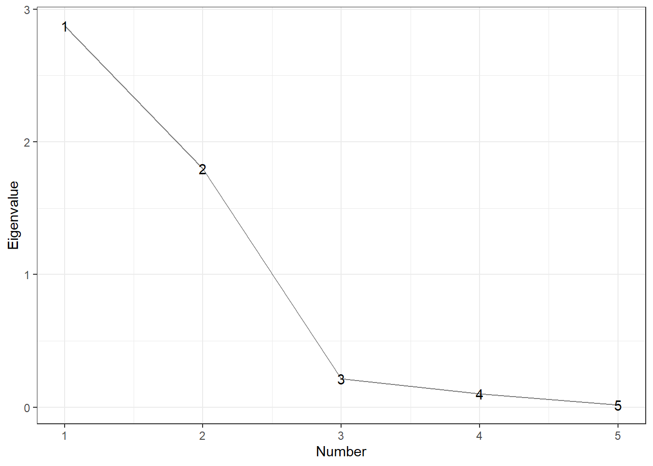

screeplot(cor_pca, type = 'lines')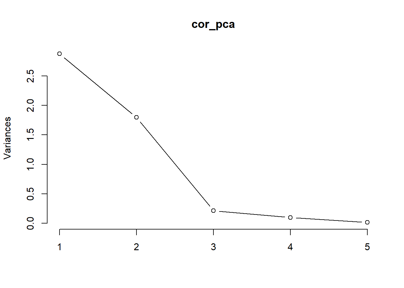

## Keep 2 factors based on scree plot and eigenvalues
factor_pca <- principal(Harman.5, nfactors = 2, rotate = "none")
factor_pca
#> Principal Components Analysis
#> Call: principal(r = Harman.5, nfactors = 2, rotate = "none")
#> Standardized loadings (pattern matrix) based upon correlation matrix
#>               PC1   PC2   h2    u2 com
#> population   0.58  0.81 0.99 0.012 1.8
#> schooling    0.77 -0.54 0.89 0.115 1.8
#> employment   0.67  0.73 0.98 0.021 2.0
#> professional 0.93 -0.10 0.88 0.120 1.0
#> housevalue   0.79 -0.56 0.94 0.062 1.8
#> 
#>                        PC1  PC2
#> SS loadings           2.87 1.80
#> Proportion Var        0.57 0.36
#> Cumulative Var        0.57 0.93
#> Proportion Explained  0.62 0.38
#> Cumulative Proportion 0.62 1.00
#> 
#> Mean item complexity =  1.7
#> Test of the hypothesis that 2 components are sufficient.
#> 
#> The root mean square of the residuals (RMSR) is  0.03 
#>  with the empirical chi square  0.29  with prob <  0.59 
#> 
#> Fit based upon off diagonal values = 1

# factor 1 = overall socioeconomic health
# factor 2 = contrast of the population and employment against school and house value


## Ssquared multiple correlation (SMC) prior, no rotation
factor_pca_smc <- fa(
    Harman.5,
    nfactors = 2,
    fm = "pa",
    rotate = "none",
    SMC = TRUE
)
factor_pca_smc
#> Factor Analysis using method =  pa
#> Call: fa(r = Harman.5, nfactors = 2, rotate = "none", SMC = TRUE, fm = "pa")
#> Standardized loadings (pattern matrix) based upon correlation matrix
#>               PA1   PA2   h2      u2 com
#> population   0.62  0.78 1.00 -0.0027 1.9
#> schooling    0.70 -0.53 0.77  0.2277 1.9
#> employment   0.70  0.68 0.96  0.0413 2.0
#> professional 0.88 -0.15 0.80  0.2017 1.1
#> housevalue   0.78 -0.60 0.96  0.0361 1.9
#> 
#>                        PA1  PA2
#> SS loadings           2.76 1.74
#> Proportion Var        0.55 0.35
#> Cumulative Var        0.55 0.90
#> Proportion Explained  0.61 0.39
#> Cumulative Proportion 0.61 1.00
#> 
#> Mean item complexity =  1.7
#> Test of the hypothesis that 2 factors are sufficient.
#> 
#> df null model =  10  with the objective function =  6.38 with Chi Square =  54.25
#> df of  the model are 1  and the objective function was  0.34 
#> 
#> The root mean square of the residuals (RMSR) is  0.01 
#> The df corrected root mean square of the residuals is  0.03 
#> 
#> The harmonic n.obs is  12 with the empirical chi square  0.02  with prob <  0.88 
#> The total n.obs was  12  with Likelihood Chi Square =  2.44  with prob <  0.12 
#> 
#> Tucker Lewis Index of factoring reliability =  0.596
#> RMSEA index =  0.336  and the 90 % confidence intervals are  0 0.967
#> BIC =  -0.04
#> Fit based upon off diagonal values = 1

## SMC prior, Promax rotation
factor_pca_smc_pro <- fa(
    Harman.5,
    nfactors = 2,
    fm = "pa",
    rotate = "Promax",
    SMC = TRUE
)
factor_pca_smc_pro
#> Factor Analysis using method =  pa
#> Call: fa(r = Harman.5, nfactors = 2, rotate = "Promax", SMC = TRUE, 
#>     fm = "pa")
#> Standardized loadings (pattern matrix) based upon correlation matrix
#>                PA1   PA2   h2      u2 com
#> population   -0.11  1.02 1.00 -0.0027 1.0
#> schooling     0.90 -0.11 0.77  0.2277 1.0
#> employment    0.02  0.97 0.96  0.0413 1.0
#> professional  0.75  0.33 0.80  0.2017 1.4
#> housevalue    1.01 -0.14 0.96  0.0361 1.0
#> 
#>                        PA1  PA2
#> SS loadings           2.38 2.11
#> Proportion Var        0.48 0.42
#> Cumulative Var        0.48 0.90
#> Proportion Explained  0.53 0.47
#> Cumulative Proportion 0.53 1.00
#> 
#>  With factor correlations of 
#>      PA1  PA2
#> PA1 1.00 0.25
#> PA2 0.25 1.00
#> 
#> Mean item complexity =  1.1
#> Test of the hypothesis that 2 factors are sufficient.
#> 
#> df null model =  10  with the objective function =  6.38 with Chi Square =  54.25
#> df of  the model are 1  and the objective function was  0.34 
#> 
#> The root mean square of the residuals (RMSR) is  0.01 
#> The df corrected root mean square of the residuals is  0.03 
#> 
#> The harmonic n.obs is  12 with the empirical chi square  0.02  with prob <  0.88 
#> The total n.obs was  12  with Likelihood Chi Square =  2.44  with prob <  0.12 
#> 
#> Tucker Lewis Index of factoring reliability =  0.596
#> RMSEA index =  0.336  and the 90 % confidence intervals are  0 0.967
#> BIC =  -0.04
#> Fit based upon off diagonal values = 1

## SMC prior, varimax rotation
factor_pca_smc_var <- fa(
    Harman.5,
    nfactors = 2,
    fm = "pa",
    rotate = "varimax",
    SMC = TRUE
)
## Make a data frame of the loadings for ggplot2
factors_df <-
    bind_rows(
        data.frame(
            y = rownames(factor_pca_smc$loadings),
            unclass(factor_pca_smc$loadings)
        ),
        data.frame(
            y = rownames(factor_pca_smc_pro$loadings),
            unclass(factor_pca_smc_pro$loadings)
        ),
        data.frame(
            y = rownames(factor_pca_smc_var$loadings),
            unclass(factor_pca_smc_var$loadings)
        ),
        .id = "Rotation"
    )
flag_gg <- ggplot(factors_df) +
    geom_vline(aes(xintercept = 0)) +
    geom_hline(aes(yintercept = 0)) +
    geom_point(aes(
        x = PA2,
        y = PA1,
        col = y,
        shape = y
    ), size = 2) +
    scale_x_continuous(name = "Factor 2", limits = c(-1.1, 1.1)) +
    scale_y_continuous(name = "Factor1", limits = c(-1.1, 1.1)) +
    facet_wrap("Rotation", labeller = labeller(Rotation = c(
        "1" = "Original", "2" = "Promax", "3" = "Varimax"
    ))) +
    coord_fixed(ratio = 1) # make aspect ratio of each facet 1

flag_gg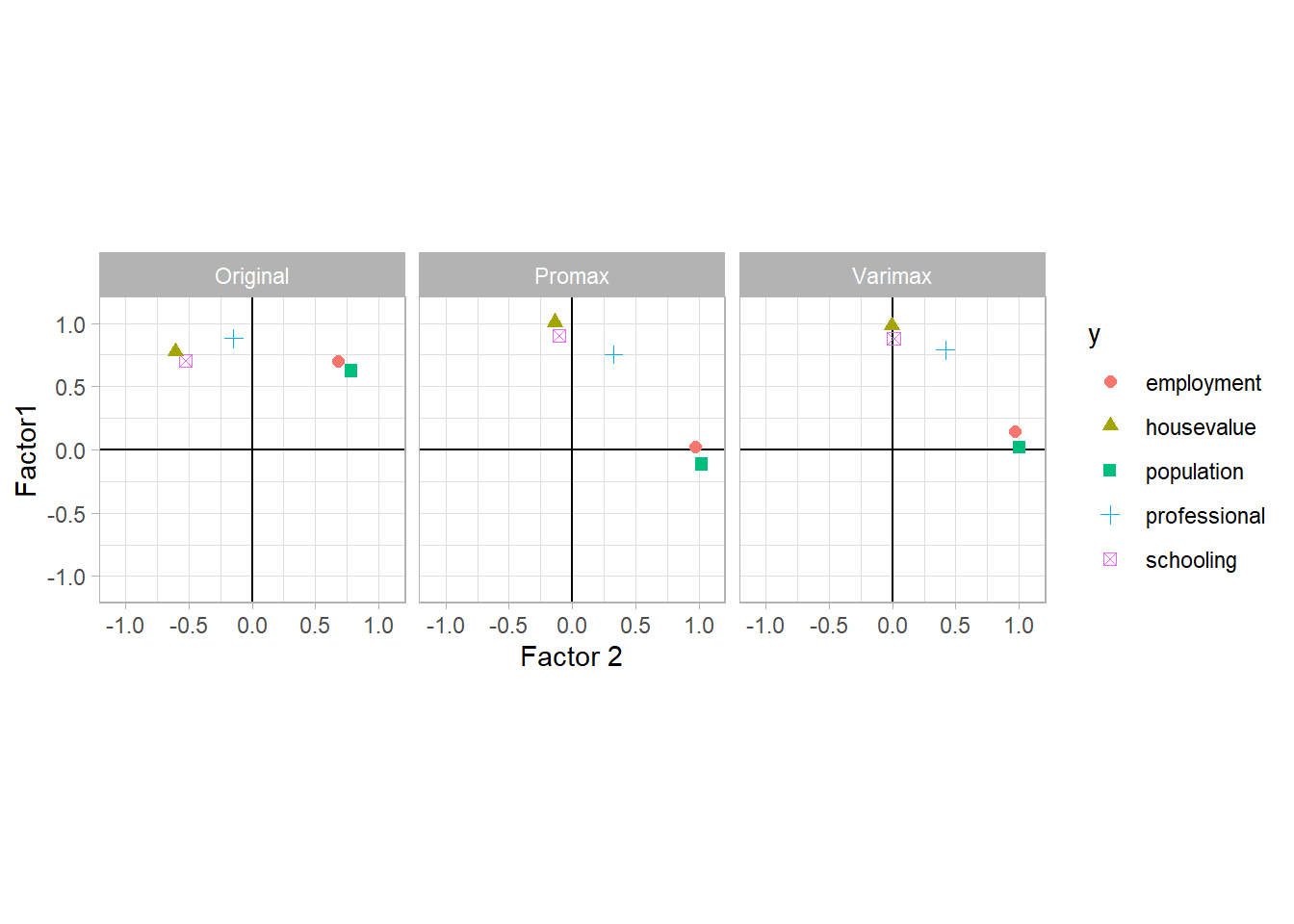

# promax and varimax did a good job to assign trait to a particular factor

factor_mle_1 <- fa(
    Harman.5,
    nfactors = 1,
    fm = "mle",
    rotate = "none",
    SMC = TRUE
)
factor_mle_1
#> Factor Analysis using method =  ml
#> Call: fa(r = Harman.5, nfactors = 1, rotate = "none", SMC = TRUE, fm = "mle")
#> Standardized loadings (pattern matrix) based upon correlation matrix
#>               ML1    h2     u2 com
#> population   0.97 0.950 0.0503   1
#> schooling    0.14 0.021 0.9791   1
#> employment   1.00 0.995 0.0049   1
#> professional 0.51 0.261 0.7388   1
#> housevalue   0.12 0.014 0.9864   1
#> 
#>                 ML1
#> SS loadings    2.24
#> Proportion Var 0.45
#> 
#> Mean item complexity =  1
#> Test of the hypothesis that 1 factor is sufficient.
#> 
#> df null model =  10  with the objective function =  6.38 with Chi Square =  54.25
#> df of  the model are 5  and the objective function was  3.14 
#> 
#> The root mean square of the residuals (RMSR) is  0.41 
#> The df corrected root mean square of the residuals is  0.57 
#> 
#> The harmonic n.obs is  12 with the empirical chi square  39.41  with prob <  2e-07 
#> The total n.obs was  12  with Likelihood Chi Square =  24.56  with prob <  0.00017 
#> 
#> Tucker Lewis Index of factoring reliability =  0.022
#> RMSEA index =  0.564  and the 90 % confidence intervals are  0.374 0.841
#> BIC =  12.14
#> Fit based upon off diagonal values = 0.5
#> Measures of factor score adequacy             
#>                                                    ML1
#> Correlation of (regression) scores with factors   1.00
#> Multiple R square of scores with factors          1.00
#> Minimum correlation of possible factor scores     0.99

factor_mle_2 <- fa(
    Harman.5,
    nfactors = 2,
    fm = "mle",
    rotate = "none",
    SMC = TRUE
)
factor_mle_2
#> Factor Analysis using method =  ml
#> Call: fa(r = Harman.5, nfactors = 2, rotate = "none", SMC = TRUE, fm = "mle")
#> Standardized loadings (pattern matrix) based upon correlation matrix
#>                ML2  ML1   h2    u2 com
#> population   -0.03 1.00 1.00 0.005 1.0
#> schooling     0.90 0.04 0.81 0.193 1.0
#> employment    0.09 0.98 0.96 0.036 1.0
#> professional  0.78 0.46 0.81 0.185 1.6
#> housevalue    0.96 0.05 0.93 0.074 1.0
#> 
#>                        ML2  ML1
#> SS loadings           2.34 2.16
#> Proportion Var        0.47 0.43
#> Cumulative Var        0.47 0.90
#> Proportion Explained  0.52 0.48
#> Cumulative Proportion 0.52 1.00
#> 
#> Mean item complexity =  1.1
#> Test of the hypothesis that 2 factors are sufficient.
#> 
#> df null model =  10  with the objective function =  6.38 with Chi Square =  54.25
#> df of  the model are 1  and the objective function was  0.31 
#> 
#> The root mean square of the residuals (RMSR) is  0.01 
#> The df corrected root mean square of the residuals is  0.05 
#> 
#> The harmonic n.obs is  12 with the empirical chi square  0.05  with prob <  0.82 
#> The total n.obs was  12  with Likelihood Chi Square =  2.22  with prob <  0.14 
#> 
#> Tucker Lewis Index of factoring reliability =  0.658
#> RMSEA index =  0.307  and the 90 % confidence intervals are  0 0.945
#> BIC =  -0.26
#> Fit based upon off diagonal values = 1
#> Measures of factor score adequacy             
#>                                                    ML2  ML1
#> Correlation of (regression) scores with factors   0.98 1.00
#> Multiple R square of scores with factors          0.95 1.00
#> Minimum correlation of possible factor scores     0.91 0.99

factor_mle_3 <- fa(
    Harman.5,
    nfactors = 3,
    fm = "mle",
    rotate = "none",
    SMC = TRUE
)
factor_mle_3
#> Factor Analysis using method =  ml
#> Call: fa(r = Harman.5, nfactors = 3, rotate = "none", SMC = TRUE, fm = "mle")
#> Standardized loadings (pattern matrix) based upon correlation matrix
#>                ML2  ML1   ML3   h2     u2 com
#> population   -0.12 0.98 -0.11 0.98 0.0162 1.1
#> schooling     0.89 0.15  0.29 0.90 0.0991 1.3
#> employment    0.00 1.00  0.04 0.99 0.0052 1.0
#> professional  0.72 0.52 -0.10 0.80 0.1971 1.9
#> housevalue    0.97 0.13 -0.09 0.97 0.0285 1.1
#> 
#>                        ML2  ML1  ML3
#> SS loadings           2.28 2.26 0.11
#> Proportion Var        0.46 0.45 0.02
#> Cumulative Var        0.46 0.91 0.93
#> Proportion Explained  0.49 0.49 0.02
#> Cumulative Proportion 0.49 0.98 1.00
#> 
#> Mean item complexity =  1.2
#> Test of the hypothesis that 3 factors are sufficient.
#> 
#> df null model =  10  with the objective function =  6.38 with Chi Square =  54.25
#> df of  the model are -2  and the objective function was  0 
#> 
#> The root mean square of the residuals (RMSR) is  0 
#> The df corrected root mean square of the residuals is  NA 
#> 
#> The harmonic n.obs is  12 with the empirical chi square  0  with prob <  NA 
#> The total n.obs was  12  with Likelihood Chi Square =  0  with prob <  NA 
#> 
#> Tucker Lewis Index of factoring reliability =  1.318
#> Fit based upon off diagonal values = 1
#> Measures of factor score adequacy             
#>                                                    ML2  ML1  ML3
#> Correlation of (regression) scores with factors   0.99 1.00 0.82
#> Multiple R square of scores with factors          0.98 1.00 0.68
#> Minimum correlation of possible factor scores     0.96 0.99 0.36

The output info for the null hypothesis of no common factors is in the statement “The degrees of freedom for the null model ..”

The output info for the null hypothesis that number of factors is sufficient is in the statement “The total number of observations was …”

One factor is not enough, two is sufficient, and not enough data for 3 factors (df of -2 and NA for p-value). Hence, we should use 2-factor model.

22.4 Discriminant Analysis

Suppose we have two or more different populations from which observations could come from. Discriminant analysis seeks to determine which of the possible population an observation comes from while making as few mistakes as possible

• This is an alternative to logistic approaches with the following advantages:

  • when there is clear separation between classes, the parameter estimates for the logic regression model can be surprisingly unstable, while discriminant approaches do not suffer

  • If X is normal in each of the classes and the sample size is small, then discriminant approaches can be more accurate

Notation

Similar to MANOVA, let \(\mathbf{y}_{j1},\mathbf{y}_{j2},\dots, \mathbf{y}_{in_j} \sim iid f_j (\mathbf{y})\) for \(j = 1,\dots, h\)

Let \(f_j(\mathbf{y})\) be the density function for population j . Note that each vector \(\mathbf{y}\) contain measurements on all \(p\) traits

1. Assume that each observation is from one of \(h\) possible populations.
2. We want to form a discriminant rule that will allocate an observation \(\mathbf{y}\) to population j when \(\mathbf{y}\) is in fact from this population

22.4.1 Known Populations

The maximum likelihood discriminant rule for assigning an observation \(\mathbf{y}\) to one of the \(h\) populations allocates \(\mathbf{y}\) to the population that gives the largest likelihood to \(\mathbf{y}\)

Consider the likelihood for a single observation \(\mathbf{y}\), which has the form \(f_j (\mathbf{y})\) where j is the true population.

Since \(j\) is unknown, to make the likelihood as large as possible, we should choose the value j which causes \(f_j (\mathbf{y})\) to be as large as possible

Consider a simple univariate example. Suppose we have data from one of two binomial populations.

• The first population has \(n= 10\) trials with success probability \(p = .5\)

• The second population has \(n= 10\) trials with success probability \(p = .7\)

• to which population would we assign an observation of \(y = 7\)

• Note:

  • \(f(y = 7|n = 10, p = .5) = .117\)

  • \(f(y = 7|n = 10, p = .7) = .267\) where \(f(.)\) is the binomial likelihood.

  • Hence, we choose the second population

Another example

We have 2 populations, where

• First population: \(N(\mu_1, \sigma^2_1)\)

• Second population: \(N(\mu_2, \sigma^2_2)\)

The likelihood for a single observation is

\[ f_j (y) = (2\pi \sigma^2_j)^{-1/2} \exp\{ -\frac{1}{2}(\frac{y - \mu_j}{\sigma_j})^2\} \]

Consider a likelihood ratio rule

\[ \begin{aligned} \Lambda &= \frac{\text{likelihood of y from pop 1}}{\text{likelihood of y from pop 2}} \\ &= \frac{f_1(y)}{f_2(y)} \\ &= \frac{\sigma_2}{\sigma_1} \exp\{-\frac{1}{2}[(\frac{y - \mu_1}{\sigma_1})^2- (\frac{y - \mu_2}{\sigma_2})^2] \} \end{aligned} \]

Hence, we classify into

• pop 1 if \(\Lambda >1\)

• pop 2 if \(\Lambda <1\)

• for ties, flip a coin

Another way to think:

we classify into population 1 if the “standardized distance” of y from \(\mu_1\) is less than the “standardized distance” of y from \(\mu_2\) which is referred to as a quadratic discriminant rule.

(Significant simplification occurs in th special case where \(\sigma_1 = \sigma_2 = \sigma^2\))

Thus, we classify into population 1 if

\[ (y - \mu_2)^2 > (y - \mu_1)^2 \]

or

\[ |y- \mu_2| > |y - \mu_1| \]

and

\[ -2 \log (\Lambda) = -2y \frac{(\mu_1 - \mu_2)}{\sigma^2} + \frac{(\mu_1^2 - \mu_2^2)}{\sigma^2} = \beta y + \alpha \]

Thus, we classify into population 1 if this is less than 0.

Discriminant classification rule is linear in y in this case.

22.4.1.1 Multivariate Expansion

Suppose that there are 2 populations

• \(N_p(\mathbf{\mu}_1, \mathbf{\Sigma}_1)\)

• \(N_p(\mathbf{\mu}_2, \mathbf{\Sigma}_2)\)

\[ \begin{aligned} -2 \log(\frac{f_1 (\mathbf{x})}{f_2 (\mathbf{x})}) &= \log|\mathbf{\Sigma}_1| + (\mathbf{x} - \mathbf{\mu}_1)' \mathbf{\Sigma}^{-1}_1 (\mathbf{x} - \mathbf{\mu}_1) \\ &- [\log|\mathbf{\Sigma}_2|+ (\mathbf{x} - \mathbf{\mu}_2)' \mathbf{\Sigma}^{-1}_2 (\mathbf{x} - \mathbf{\mu}_2) ] \end{aligned} \]

Again, we classify into population 1 if this is less than 0, otherwise, population 2. And like the univariate case with non-equal variances, this is a quadratic discriminant rule.

And if the covariance matrices are equal: \(\mathbf{\Sigma}_1 = \mathbf{\Sigma}_2 = \mathbf{\Sigma}_1\) classify into population 1 if

\[ (\mathbf{\mu}_1 - \mathbf{\mu}_2)' \mathbf{\Sigma}^{-1}\mathbf{x} - \frac{1}{2} (\mathbf{\mu}_1 - \mathbf{\mu}_2)' \mathbf{\Sigma}^{-1} (\mathbf{\mu}_1 - \mathbf{\mu}_2) \ge 0 \]

This linear discriminant rule is also referred to as Fisher’s linear discriminant function

By assuming the covariance matrices are equal, we assume that the shape and orientation fo the two populations must be the same (which can be a strong restriction)

In other words, for each variable, it can have different mean but the same variance.

• Note: LDA Bayes decision boundary is linear. Hence, quadratic decision boundary might lead to better classification. Moreover, the assumption of same variance/covariance matrix across all classes for Gaussian densities imposes the linear rule, if we allow the predictors in each class to follow MVN distribution with class-specific mean vectors and variance/covariance matrices, then it is Quadratic Discriminant Analysis. But then, you will have more parameters to estimate (which gives more flexibility than LDA) at the cost of more variance (bias -variance tradeoff).

When \(\mathbf{\mu}_1, \mathbf{\mu}_2, \mathbf{\Sigma}\) are known, the probability of misclassification can be determined:

\[ \begin{aligned} P(2|1) &= P(\text{calssify into pop 2| x is from pop 1}) \\ &= P((\mathbf{\mu}_1 - \mathbf{\mu}_2)' \mathbf{\Sigma}^{-1} \mathbf{x} \le \frac{1}{2} (\mathbf{\mu}_1 - \mathbf{\mu}_2)' \mathbf{\Sigma}^{-1} (\mathbf{\mu}_1 - \mathbf{\mu}_2)|\mathbf{x} \sim N(\mu_1, \mathbf{\Sigma}) \\ &= \Phi(-\frac{1}{2} \delta) \end{aligned} \]

where

• \(\delta^2 = (\mathbf{\mu}_1 - \mathbf{\mu}_2)' \mathbf{\Sigma}^{-1} (\mathbf{\mu}_1 - \mathbf{\mu}_2)\)

• \(\Phi\) is the standard normal CDF

Suppose there are \(h\) possible populations, which are distributed as \(N_p (\mathbf{\mu}_p, \mathbf{\Sigma})\). Then, the maximum likelihood (linear) discriminant rule allocates \(\mathbf{y}\) to population j where j minimizes the squared Mahalanobis distance

\[ (\mathbf{y} - \mathbf{\mu}_j)' \mathbf{\Sigma}^{-1} (\mathbf{y} - \mathbf{\mu}_j) \]

22.4.1.2 Bayes Discriminant Rules

If we know that population j has prior probabilities \(\pi_j\) (assume \(\pi_j >0\)) we can form the Bayes discriminant rule.

This rule allocates an observation \(\mathbf{y}\) to the population for which \(\pi_j f_j (\mathbf{y})\) is maximized.

Note:

• Maximum likelihood discriminant rule is a special case of the Bayes discriminant rule, where it sets all the \(\pi_j = 1/h\)

Optimal Properties of Bayes Discriminant Rules

• let \(p_{ii}\) be the probability of correctly assigning an observation from population i

• then one rule (with probabilities \(p_{ii}\) ) is as good as another rule (with probabilities \(p_{ii}'\) ) if \(p_{ii} \ge p_{ii}'\) for all \(i = 1,\dots, h\)

• The first rule is better than the alternative if \(p_{ii} > p_{ii}'\) for at least one i.

• A rule for which there is no better alternative is called admissible

• Bayes Discriminant Rules are admissible

• If we utilized prior probabilities, then we can form the posterior probability of a correct allocation, \(\sum_{i=1}^h \pi_i p_{ii}\)

• Bayes Discriminant Rules have the largest possible posterior probability of correct allocation with respect to the prior

• These properties show that Bayes Discriminant rule is our best approach.

Unequal Cost

• We want to consider the cost misallocation

  • Define \(c_{ij}\) to be the cost associated with allocation a member of population j to population i.

• Assume that

  • \(c_{ij} >0\) for all \(i \neq j\)

  • \(c_{ij} = 0\) if \(i = j\)

• We could determine the expected amount of loss for an observation allocated to population i as \(\sum_j c_{ij} p_{ij}\) where the \(p_{ij}s\) are the probabilities of allocating an observation from population j into population i

• We want to minimize the amount of loss expected for our rule. Using a Bayes Discrimination, allocate \(\mathbf{y}\) to the population j which minimizes \(\sum_{k \neq j} c_{ij} \pi_k f_k(\mathbf{y})\)

• We could assign equal probabilities to each group and get a maximum likelihood type rule. here, we would allocate \(\mathbf{y}\) to population j which minimizes \(\sum_{k \neq j}c_{jk} f_k(\mathbf{y})\)

Example:

Two binomial populations, each of size 10, with probabilities \(p_1 = .5\) and \(p_2 = .7\)

And the probability of being in the first population is .9

However, suppose the cost of inappropriately allocating into the first population is 1 and the cost of incorrectly allocating into the second population is 5.

In this case, we pick population 1 over population 2

In general, we consider two regions, \(R_1\) and \(R_2\) associated with population 1 and 2:

\[ R_1: \frac{f_1 (\mathbf{x})}{f_2 (\mathbf{x})} \ge \frac{c_{12} \pi_2}{c_{21} \pi_1} \]

\[ R_2: \frac{f_1 (\mathbf{x})}{f_2 (\mathbf{x})} < \frac{c_{12} \pi_2}{c_{21} \pi_1} \]

where \(c_{12}\) is the cost of assigning a member of population 2 to population 1.

22.4.1.3 Discrimination Under Estimation

Suppose we know the form of the distributions for populations of interests, but we still have to estimate the parameters.

Example:

we know the distributions are multivariate normal, but we have to estimate the means and variances

The maximum likelihood discriminant rule allocates an observation \(\mathbf{y}\) to population j when j maximizes the function

\[ f_j (\mathbf{y} |\hat{\theta}) \]

where \(\hat{\theta}\) are the maximum likelihood estimates of the unknown parameters

For instance, we have 2 multivariate normal populations with distinct means, but common variance covariance matrix

MLEs for \(\mathbf{\mu}_1\) and \(\mathbf{\mu}_2\) are \(\mathbf{\bar{y}}_1\) and \(\mathbf{\bar{y}}_2\)and common \(\mathbf{\Sigma}\) is \(\mathbf{S}\).

Thus, an estimated discriminant rule could be formed by substituting these sample values for the population values

22.4.1.4 Native Bayes

• The challenge with classification using Bayes’ is that we don’t know the (true) densities, \(f_k, k = 1, \dots, K\), while LDA and QDA make strong multivariate normality assumptions to deal with this.

• Naive Bayes makes only one assumption: within the k-th class, the p predictors are independent (i.e,, for \(k = 1,\dots, K\)

\[ f_k(x) = f_{k1}(x_1) \times f_{k2}(x_2) \times \dots \times f_{kp}(x_p) \]

where \(f_{kj}\) is the density function of the j-th predictor among observation in the k-th class.

This assumption allows the use of joint distribution without the need to account for dependence between observations. However, this (native) assumption can be unrealistic, but still works well in cases where the number of sample (n) is not large relative to the number of features (p).

With this assumption, we have

\[ P(Y=k|X=x) = \frac{\pi_k \times f_{k1}(x_1) \times \dots \times f_{kp}(x_p)}{\sum_{l=1}^K \pi_l \times f_{l1}(x_1)\times \dots f_{lp}(x_p)} \]

we only need to estimate the one-dimensional density function \(f_{kj}\) with either of these approaches:

• When \(X_j\) is quantitative, assume it has a univariate normal distribution (with independence): \(X_j | Y = k \sim N(\mu_{jk}, \sigma^2_{jk})\) which is more restrictive than QDA because it assumes predictors are independent (e.g., a diagonal covariance matrix)

• When \(X_j\) is quantitative, use a kernel density estimator Kernel Methods ; which is a smoothed histogram

• When \(X_j\) is qualitative, we count the promotion of training observations for the j-th predictor corresponding to each class.

22.4.1.5 Comparison of Classification Methods

Assuming we have K classes and K is the baseline from (James , Witten, Hastie, and Tibshirani book)

Comparing the log odds relative to the K class

22.4.1.5.1 Logistic Regression

\[ \log(\frac{P(Y=k|X = x)}{P(Y = K| X = x)}) = \beta_{k0} + \sum_{j=1}^p \beta_{kj}x_j \]

22.4.1.5.2 LDA

\[ \log(\frac{P(Y = k | X = x)}{P(Y = K | X = x)} = a_k + \sum_{j=1}^p b_{kj} x_j \]

where \(a_k\) and \(b_{kj}\) are functions of \(\pi_k, \pi_K, \mu_k , \mu_K, \mathbf{\Sigma}\)

Similar to logistic regression, LDA assumes the log odds is linear in \(x\)

Even though they look like having the same form, the parameters in logistic regression are estimated by MLE, where as LDA linear parameters are specified by the prior and normal distributions

We expect LDA to outperform logistic regression when the normality assumption (approximately) holds, and logistic regression to perform better when it does not

22.4.1.5.3 QDA

\[ \log(\frac{P(Y=k|X=x}{P(Y=K | X = x}) = a_k + \sum_{j=1}^{p}b_{kj}x_{j} + \sum_{j=1}^p \sum_{l=1}^p c_{kjl}x_j x_l \]

where \(a_k, b_{kj}, c_{kjl}\) are functions \(\pi_k , \pi_K, \mu_k, \mu_K ,\mathbf{\Sigma}_k, \mathbf{\Sigma}_K\)

22.4.1.5.4 Naive Bayes

\[ \log (\frac{P(Y = k | X = x)}{P(Y = K | X = x}) = a_k + \sum_{j=1}^p g_{kj} (x_j) \]

where \(a_k = \log (\pi_k / \pi_K)\) and \(g_{kj}(x_j) = \log(\frac{f_{kj}(x_j)}{f_{Kj}(x_j)})\) which is the form of generalized additive model

22.4.1.5.5 Summary

• LDA is a special case of QDA

• LDA is robust when it comes to high dimensions

• Any classifier with a linear decision boundary is a special case of naive Bayes with \(g_{kj}(x_j) = b_{kj} x_j\), which means LDA is a special case of naive Bayes. LDA assumes that the features are normally distributed with a common within-class covariance matrix, and naive Bayes assumes independence of the features.

• Naive bayes is also a special case of LDA with \(\mathbf{\Sigma}\) restricted to a diagonal matrix with diagonals, \(\sigma^2\) (another notation \(diag (\mathbf{\Sigma})\) ) assuming \(f_{kj}(x_j) = N(\mu_{kj}, \sigma^2_j)\)

• QDA and naive Bayes are not special case of each other. In principal,e naive Bayes can produce a more flexible fit by the choice of \(g_{kj}(x_j)\) , but it’s restricted to only purely additive fit, but QDA includes multiplicative terms of the form \(c_{kjl}x_j x_l\)

• None of these methods uniformly dominates the others: the choice of method depends on the true distribution of the predictors in each of the K classes, n and p (i.e., related to the bias-variance tradeoff).

Compare to the non-parametric method (KNN)

• KNN would outperform both LDA and logistic regression when the decision boundary is highly nonlinear, but can’t say which predictors are most important, and requires many observations

• KNN is also limited in high-dimensions due to the curse of dimensionality

• Since QDA is a special type of nonlinear decision boundary (quadratic), it can be considered as a compromise between the linear methods and KNN classification. QDA can have fewer training observations than KNN but not as flexible.

From simulation:

True decision boundary	Best performance
Linear	LDA + Logistic regression
Moderately nonlinear	QDA + Naive Bayes
Highly nonlinear (many training, p is not large)	KNN

• like linear regression, we can also introduce flexibility by including transformed features \(\sqrt{X}, X^2, X^3\)

22.4.2 Probabilities of Misclassification

When the distribution are exactly known, we can determine the misclassification probabilities exactly. however, when we need to estimate the population parameters, we have to estimate the probability of misclassification

• Naive method

  • Plugging the parameters estimates into the form for the misclassification probabilities results to derive at the estimates of the misclassification probability.

  • But this will tend to be optimistic when the number of samples in one or more populations is small.

• Resubstitution method

  • Use the proportion of the samples from population i that would be allocated to another population as an estimate of the misclassification probability

  • But also optimistic when the number of samples is small

• Jack-knife estimates:

  • The above two methods use observation to estimate both parameters and also misclassification probabilities based upon the discriminant rule

  • Alternatively, we determine the discriminant rule based upon all of the data except the k-th observation from the j-th population

  • then, determine if the k-th observation would be misclassified under this rule

  • perform this process for all \(n_j\) observation in population j . An estimate fo the misclassification probability would be the fraction of \(n_j\) observations which were misclassified

  • repeat the process for other \(i \neq j\) populations

  • This method is more reliable than the others, but also computationally intensive

• Cross-Validation

Summary

Consider the group-specific densities \(f_j (\mathbf{x})\) for multivariate vector \(\mathbf{x}\).

Assume equal misclassifications costs, the Bayes classification probability of \(\mathbf{x}\) belonging to the j-th population is

\[ p(j |\mathbf{x}) = \frac{\pi_j f_j (\mathbf{x})}{\sum_{k=1}^h \pi_k f_k (\mathbf{x})} \]

\(j = 1,\dots, h\)

where there are \(h\) possible groups.

We then classify into the group for which this probability of membership is largest

Alternatively, we can write this in terms of a generalized squared distance formation

\[ D_j^2 (\mathbf{x}) = d_j^2 (\mathbf{x})+ g_1(j) + g_2 (j) \]

where

• \(d_j^2(\mathbf{x}) = (\mathbf{x} - \mathbf{\mu}_j)' \mathbf{V}_j^{-1} (\mathbf{x} - \mathbf{\mu}_j)\) is the squared Mahalanobis distance from \(\mathbf{x}\) to the centroid of group j, and

  • \(\mathbf{V}_j = \mathbf{S}_j\) if the within group covariance matrices are not equal

  • \(\mathbf{V}_j = \mathbf{S}_p\) if a pooled covariance estimate is appropriate

and

\[ g_1(j) = \begin{cases} \ln |\mathbf{S}_j| & \text{within group covariances are not equal} \\ 0 & \text{pooled covariance} \end{cases} \]

\[ g_2(j) = \begin{cases} -2 \ln \pi_j & \text{prior probabilities are not equal} \\ 0 & \text{prior probabilities are equal} \end{cases} \]

then, the posterior probability of belonging to group j is

\[ p(j| \mathbf{x}) = \frac{\exp(-.5 D_j^2(\mathbf{x}))}{\sum_{k=1}^h \exp(-.5 D^2_k (\mathbf{x}))} \]

where \(j = 1,\dots , h\)

and \(\mathbf{x}\) is classified into group j if \(p(j | \mathbf{x})\) is largest for \(j = 1,\dots,h\) (or, \(D_j^2(\mathbf{x})\) is smallest).

22.4.2.1 Assessing Classification Performance

For binary classification, confusion matrix

	Predicted class
		- or Null	+ or Null	Total
True Class	- or Null	True Neg (TN)	False Pos (FP)	N
	+ or Null	False Neg (FN)	True Pos (TP)	P
	Total	N*	P*

and table 4.6 from (James et al. 2013)

Name	Definition	Synonyms
False Pos rate	FP/N	Type I error, 1 0 Specificity
True Pos. rate	TP/P	1 - Type II error, power, sensitivity, recall
Pos Pred. value	TP/P*	Precision, 1 - false discovery promotion
Neg. Pred. value	TN/N*

ROC curve (receiver Operating Characteristics) is a graphical comparison between sensitivity (true positive) and specificity ( = 1 - false positive)

y-axis = true positive rate

x-axis = false positive rate

as we change the threshold rate for classifying an observation as from 0 to 1

AUC (area under the ROC) ideally would equal to 1, a bad classifier would have AUC = 0.5 (pure chance)

22.4.3 Unknown Populations/ Nonparametric Discrimination

When your multivariate data are not Gaussian, or known distributional form at all, we can use the following methods

22.4.3.1 Kernel Methods

We approximate \(f_j (\mathbf{x})\) by a kernel density estimate

\[ \hat{f}_j(\mathbf{x}) = \frac{1}{n_j} \sum_{i = 1}^{n_j} K_j (\mathbf{x} - \mathbf{x}_i) \]

where

• \(K_j (.)\) is a kernel function satisfying \(\int K_j(\mathbf{z})d\mathbf{z} =1\)

• \(\mathbf{x}_i\) , \(i = 1,\dots , n_j\) is a random sample from the j-th population.

Thus, after finding \(\hat{f}_j (\mathbf{x})\) for each of the \(h\) populations, the posterior probability of group membership is

\[ p(j |\mathbf{x}) = \frac{\pi_j \hat{f}_j (\mathbf{x})}{\sum_{k-1}^h \pi_k \hat{f}_k (\mathbf{x})} \]

where \(j = 1,\dots, h\)

There are different choices for the kernel function:

• Uniform

• Normal

• Epanechnikov

• Biweight

• Triweight

We these kernels, we have to pick the “radius” (or variance, width, window width, bandwidth) of the kernel, which is a smoothing parameter (the larger the radius, the more smooth the kernel estimate of the density).

To select the smoothness parameter, we can use the following method

If we believe the populations were close to multivariate normal, then

\[ R = (\frac{4/(2p+1)}{n_j})^{1/(p+1} \]

But since we do not know for sure, we might choose several different values and select one that vies the best out of sample or cross-validation discrimination.

Moreover, you also have to decide whether to use different kernel smoothness for different populations, which is similar to the individual and pooled covariances in the classical methodology.

22.4.3.2 Nearest Neighbor Methods

The nearest neighbor (also known as k-nearest neighbor) method performs the classification of a new observation vector based on the group membership of its nearest neighbors. In practice, we find

\[ d_{ij}^2 (\mathbf{x}, \mathbf{x}_i) = (\mathbf{x}, \mathbf{x}_i) V_j^{-1}(\mathbf{x}, \mathbf{x}_i) \]

which is the distance between the vector \(\mathbf{x}\) and the \(i\)-th observation in group \(j\)

We consider different choices for \(\mathbf{V}_j\)

For example,

\[ \begin{aligned} \mathbf{V}_j &= \mathbf{S}_p \\ \mathbf{V}_j &= \mathbf{S}_j \\ \mathbf{V}_j &= \mathbf{I} \\ \mathbf{V}_j &= diag (\mathbf{S}_p) \end{aligned} \]

We find the \(k\) observations that are closest to \(\mathbf{x}\) (where users pick \(k\)). Then we classify into the most common population, weighted by the prior.

22.4.3.3 Modern Discriminant Methods

Note:

Logistic regression (with or without random effects) is a flexible model-based procedure for classification between two populations.

The extension of logistic regression to the multi-group setting is polychotomous logistic regression (or, mulinomial regression).

The machine learning and pattern recognition are growing with strong focus on nonlinear discriminant analysis methods such as:

• radial basis function networks

• support vector machines

• multiplayer perceptrons (neural networks)

The general framework

\[ g_j (\mathbf{x}) = \sum_{l = 1}^m w_{jl}\phi_l (\mathbf{x}; \mathbf{\theta}_l) + w_{j0} \]

where

• \(j = 1,\dots, h\)

• \(m\) nonlinear basis functions \(\phi_l\), each of which has \(n_m\) parameters given by \(\theta_l = \{ \theta_{lk}: k = 1, \dots , n_m \}\)

We assign \(\mathbf{x}\) to the \(j\)-th population if \(g_j(\mathbf{x})\) is the maximum for all \(j = 1,\dots, h\)

Development usually focuses on the choice and estimation of the basis functions, \(\phi_l\) and the estimation of the weights \(w_{jl}\)

More details can be found (Webb, Copsey, and Cawley 2011)

22.4.4 Application

library(class)
library(klaR)
library(MASS)
library(tidyverse)

## Read in the data
crops <- read.table("images/crops.txt")
names(crops) <- c("crop", "y1", "y2", "y3", "y4")
str(crops)
#> 'data.frame':    36 obs. of  5 variables:
#>  $ crop: chr  "Corn" "Corn" "Corn" "Corn" ...
#>  $ y1  : int  16 15 16 18 15 15 12 20 24 21 ...
#>  $ y2  : int  27 23 27 20 15 32 15 23 24 25 ...
#>  $ y3  : int  31 30 27 25 31 32 16 23 25 23 ...
#>  $ y4  : int  33 30 26 23 32 15 73 25 32 24 ...


## Read in test data
crops_test <- read.table("images/crops_test.txt")
names(crops_test) <- c("crop", "y1", "y2", "y3", "y4")
str(crops_test)
#> 'data.frame':    5 obs. of  5 variables:
#>  $ crop: chr  "Corn" "Soybeans" "Cotton" "Sugarbeets" ...
#>  $ y1  : int  16 21 29 54 32
#>  $ y2  : int  27 25 24 23 32
#>  $ y3  : int  31 23 26 21 62
#>  $ y4  : int  33 24 28 54 16

22.4.4.1 LDA

Default prior is proportional to sample size and lda and qda do not fit a constant or intercept term

## Linear discriminant analysis
lda_mod <- lda(crop ~ y1 + y2 + y3 + y4,
               data = crops)
lda_mod
#> Call:
#> lda(crop ~ y1 + y2 + y3 + y4, data = crops)
#> 
#> Prior probabilities of groups:
#>     Clover       Corn     Cotton   Soybeans Sugarbeets 
#>  0.3055556  0.1944444  0.1666667  0.1666667  0.1666667 
#> 
#> Group means:
#>                  y1       y2       y3       y4
#> Clover     46.36364 32.63636 34.18182 36.63636
#> Corn       15.28571 22.71429 27.42857 33.14286
#> Cotton     34.50000 32.66667 35.00000 39.16667
#> Soybeans   21.00000 27.00000 23.50000 29.66667
#> Sugarbeets 31.00000 32.16667 20.00000 40.50000
#> 
#> Coefficients of linear discriminants:
#>              LD1          LD2         LD3          LD4
#> y1 -6.147360e-02  0.009215431 -0.02987075 -0.014680566
#> y2 -2.548964e-02  0.042838972  0.04631489  0.054842132
#> y3  1.642126e-02 -0.079471595  0.01971222  0.008938745
#> y4  5.143616e-05 -0.013917423  0.05381787 -0.025717667
#> 
#> Proportion of trace:
#>    LD1    LD2    LD3    LD4 
#> 0.7364 0.1985 0.0576 0.0075

## Look at accuracy on the training data
lda_fitted <- predict(lda_mod,newdata = crops)
# Contingency table
lda_table <- table(truth = crops$crop, fitted = lda_fitted$class)
lda_table
#>             fitted
#> truth        Clover Corn Cotton Soybeans Sugarbeets
#>   Clover          6    0      3        0          2
#>   Corn            0    6      0        1          0
#>   Cotton          3    0      1        2          0
#>   Soybeans        0    1      1        3          1
#>   Sugarbeets      1    1      0        2          2
# accuracy of 0.5 is just random (not good)

## Posterior probabilities of membership
crops_post <- cbind.data.frame(crops,
                               crop_pred = lda_fitted$class,
                               lda_fitted$posterior)
crops_post <- crops_post %>%
    mutate(missed = crop != crop_pred)
head(crops_post)
#>   crop y1 y2 y3 y4 crop_pred     Clover      Corn    Cotton  Soybeans
#> 1 Corn 16 27 31 33      Corn 0.08935164 0.4054296 0.1763189 0.2391845
#> 2 Corn 15 23 30 30      Corn 0.07690181 0.4558027 0.1420920 0.2530101
#> 3 Corn 16 27 27 26      Corn 0.09817815 0.3422454 0.1365315 0.3073105
#> 4 Corn 18 20 25 23      Corn 0.10521511 0.3633673 0.1078076 0.3281477
#> 5 Corn 15 15 31 32      Corn 0.05879921 0.5753907 0.1173332 0.2086696
#> 6 Corn 15 32 32 15  Soybeans 0.09723648 0.3278382 0.1318370 0.3419924
#>   Sugarbeets missed
#> 1 0.08971545  FALSE
#> 2 0.07219340  FALSE
#> 3 0.11573442  FALSE
#> 4 0.09546233  FALSE
#> 5 0.03980738  FALSE
#> 6 0.10109590   TRUE
# posterior shows that posterior of corn membership is much higher than the prior

## LOOCV
# leave-one-out cross validation for linear discriminant analysis
# cannot run the predict function using the object with CV = TRUE 
# because it returns the within sample predictions
lda_cv <- lda(crop ~ y1 + y2 + y3 + y4,
              data = crops, CV = TRUE)
# Contingency table
lda_table_cv <- table(truth = crops$crop, fitted = lda_cv$class)
lda_table_cv
#>             fitted
#> truth        Clover Corn Cotton Soybeans Sugarbeets
#>   Clover          4    3      1        0          3
#>   Corn            0    4      1        2          0
#>   Cotton          3    0      0        2          1
#>   Soybeans        0    1      1        3          1
#>   Sugarbeets      2    1      0        2          1

## Predict the test data
lda_pred <- predict(lda_mod, newdata = crops_test)

## Make a contingency table with truth and most likely class
table(truth=crops_test$crop, predict=lda_pred$class)
#>             predict
#> truth        Clover Corn Cotton Soybeans Sugarbeets
#>   Clover          0    0      1        0          0
#>   Corn            0    1      0        0          0
#>   Cotton          0    0      0        1          0
#>   Soybeans        0    0      0        1          0
#>   Sugarbeets      1    0      0        0          0

LDA didn’t do well on both within sample and out-of-sample data.

22.4.4.2 QDA

## Quadratic discriminant analysis
qda_mod <- qda(crop ~ y1 + y2 + y3 + y4,
               data = crops)

## Look at accuracy on the training data
qda_fitted <- predict(qda_mod, newdata = crops)
# Contingency table
qda_table <- table(truth = crops$crop, fitted = qda_fitted$class)
qda_table
#>             fitted
#> truth        Clover Corn Cotton Soybeans Sugarbeets
#>   Clover          9    0      0        0          2
#>   Corn            0    7      0        0          0
#>   Cotton          0    0      6        0          0
#>   Soybeans        0    0      0        6          0
#>   Sugarbeets      0    0      1        1          4

## LOOCV
qda_cv <- qda(crop ~ y1 + y2 + y3 + y4,
              data = crops, CV = TRUE)
# Contingency table
qda_table_cv <- table(truth = crops$crop, fitted = qda_cv$class)
qda_table_cv
#>             fitted
#> truth        Clover Corn Cotton Soybeans Sugarbeets
#>   Clover          9    0      0        0          2
#>   Corn            3    2      0        0          2
#>   Cotton          3    0      2        0          1
#>   Soybeans        3    0      0        2          1
#>   Sugarbeets      3    0      1        1          1

## Predict the test data
qda_pred <- predict(qda_mod, newdata = crops_test)
## Make a contingency table with truth and most likely class
table(truth = crops_test$crop, predict = qda_pred$class)
#>             predict
#> truth        Clover Corn Cotton Soybeans Sugarbeets
#>   Clover          1    0      0        0          0
#>   Corn            0    1      0        0          0
#>   Cotton          0    0      1        0          0
#>   Soybeans        0    0      0        1          0
#>   Sugarbeets      0    0      0        0          1

22.4.4.3 KNN

knn uses design matrices of the features.

## Design matrices
X_train <- crops %>%
    dplyr::select(-crop)
X_test <- crops_test %>%
    dplyr::select(-crop)
Y_train <- crops$crop
Y_test <- crops_test$crop

## Nearest neighbors with 2 neighbors
knn_2 <- knn(X_train, X_train, Y_train, k = 2)
table(truth = Y_train, fitted = knn_2)
#>             fitted
#> truth        Clover Corn Cotton Soybeans Sugarbeets
#>   Clover          7    0      2        1          1
#>   Corn            0    7      0        0          0
#>   Cotton          0    0      4        0          2
#>   Soybeans        0    0      0        4          2
#>   Sugarbeets      1    0      2        0          3

## Accuracy
mean(Y_train==knn_2)
#> [1] 0.6944444

## Performance on test data
knn_2_test <- knn(X_train, X_test, Y_train, k = 2)
table(truth = Y_test, predict = knn_2_test)
#>             predict
#> truth        Clover Corn Cotton Soybeans Sugarbeets
#>   Clover          1    0      0        0          0
#>   Corn            0    1      0        0          0
#>   Cotton          0    0      0        0          1
#>   Soybeans        0    0      0        1          0
#>   Sugarbeets      0    0      0        0          1

## Accuracy
mean(Y_test==knn_2_test)
#> [1] 0.8

## Nearest neighbors with 3 neighbors
knn_3 <- knn(X_train, X_train, Y_train, k = 3)
table(truth = Y_train, fitted = knn_3)
#>             fitted
#> truth        Clover Corn Cotton Soybeans Sugarbeets
#>   Clover          8    0      1        1          1
#>   Corn            0    4      1        2          0
#>   Cotton          1    1      3        0          1
#>   Soybeans        0    1      1        4          0
#>   Sugarbeets      0    0      0        2          4

## Accuracy
mean(Y_train==knn_3)
#> [1] 0.6388889

## Performance on test data
knn_3_test <- knn(X_train, X_test, Y_train, k = 3)
table(truth = Y_test, predict = knn_3_test)
#>             predict
#> truth        Clover Corn Cotton Soybeans Sugarbeets
#>   Clover          1    0      0        0          0
#>   Corn            0    1      0        0          0
#>   Cotton          0    0      1        0          0
#>   Soybeans        0    0      0        1          0
#>   Sugarbeets      0    0      0        0          1

## Accuracy
mean(Y_test==knn_3_test)
#> [1] 1

22.4.4.4 Stepwise

Stepwise discriminant analysis using the stepclass in function in the klaR package.

step <- stepclass(
    crop ~ y1 + y2 + y3 + y4,
    data = crops,
    method = "qda",
    improvement = 0.15
)
#> correctness rate: 0.45;  in: "y1";  variables (1): y1 
#> 
#>  hr.elapsed min.elapsed sec.elapsed 
#>        0.00        0.00        0.16

step$process
#>    step var varname result.pm
#> 0 start   0      --      0.00
#> 1    in   1      y1      0.45

step$performance.measure
#> [1] "correctness rate"

Iris Data

library(dplyr)
data('iris')
set.seed(1)
samp <-
    sample.int(nrow(iris), size = floor(0.70 * nrow(iris)), replace = F)

train.iris <- iris[samp,] %>% mutate_if(is.numeric,scale)
test.iris <- iris[-samp,] %>% mutate_if(is.numeric,scale)

library(ggplot2)
iris.model <- lda(Species ~ ., data = train.iris)
#pred
pred.lda <- predict(iris.model, test.iris)
table(truth = test.iris$Species, prediction = pred.lda$class)
#>             prediction
#> truth        setosa versicolor virginica
#>   setosa         15          0         0
#>   versicolor      0         17         0
#>   virginica       0          0        13

plot(iris.model)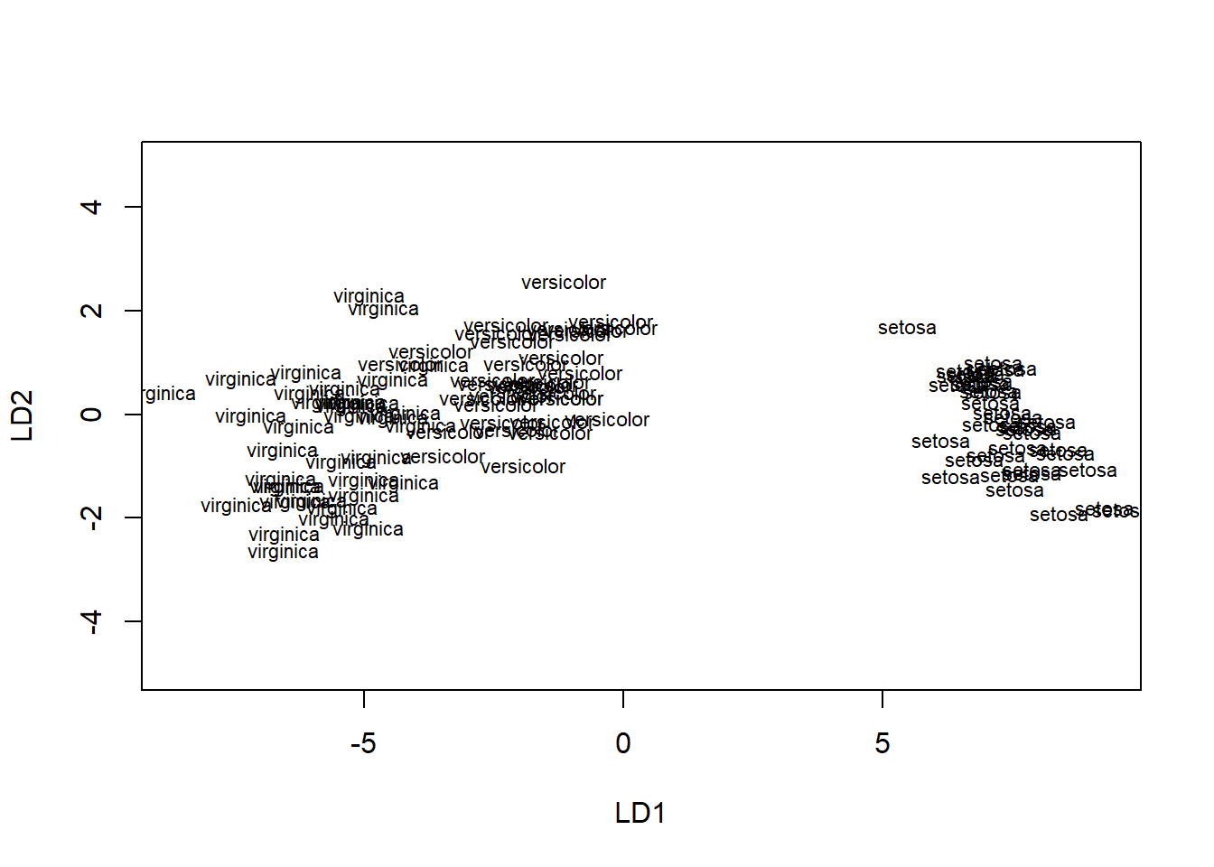

iris.model.qda <- qda(Species~.,data=train.iris)
#pred
pred.qda <- predict(iris.model.qda,test.iris)
table(truth=test.iris$Species,prediction=pred.qda$class)
#>             prediction
#> truth        setosa versicolor virginica
#>   setosa         15          0         0
#>   versicolor      0         16         1
#>   virginica       0          0        13

22.4.4.5 PCA with Discriminant Analysis

we can use both PCA for dimension reduction in discriminant analysis

zeros <- as.matrix(read.table("images/mnist0_train_b.txt"))
nines <- as.matrix(read.table("images/mnist9_train_b.txt"))
train <- rbind(zeros[1:1000, ], nines[1:1000, ])
train <- train / 255 #divide by 255 per notes (so ranges from 0 to 1)
train <- t(train) #each column is an observation
image(matrix(train[, 1], nrow = 28), main = 'Example image, unrotated')

test <- rbind(zeros[2501:3000, ], nines[2501:3000, ])
test <- test / 255
test <- t(test)
y.train <- c(rep(0, 1000), rep(9, 1000))
y.test <- c(rep(0, 500), rep(9, 500))


library(MASS)
pc <- prcomp(t(train))
train.large <- data.frame(cbind(y.train, pc$x[, 1:10]))
large <- lda(y.train ~ ., data = train.large)
#the test data set needs to be constucted w/ the same 10 princomps
test.large <- data.frame(cbind(y.test, predict(pc, t(test))[, 1:10]))
pred.lda <- predict(large, test.large)
table(truth = test.large$y.test, prediction = pred.lda$class)
#>      prediction
#> truth   0   9
#>     0 491   9
#>     9   5 495

large.qda <- qda(y.train~.,data=train.large)
#prediction
pred.qda <- predict(large.qda,test.large)
table(truth=test.large$y.test,prediction=pred.qda$class)
#>      prediction
#> truth   0   9
#>     0 493   7
#>     9   3 497