31 Matching Methods
Matching is a process that aims to close back doors - potential sources of bias - by constructing comparison groups that are similar according to a set of matching variables. This helps to ensure that any observed differences in outcomes between the treatment and comparison groups can be more confidently attributed to the treatment itself, rather than other factors that may differ between the groups.
Matching and DiD can use pre-treatment outcomes to correct for selection bias. From real world data and simulation, (Chabé-Ferret 2015) found that matching generally underestimates the average causal effect and gets closer to the true effect with more number of pre-treatment outcomes. When selection bias is symmetric around the treatment date, DID is still consistent when implemented symmetrically (i.e., the same number of period before and after treatment). In cases where selection bias is asymmetric, the MC simulations show that Symmetric DID still performs better than Matching.
Matching is useful, but not a general solution to causal problems (J. A. Smith and Todd 2005)
Assumption: Observables can identify the selection into the treatment and control groups
Identification: The exclusion restriction can be met conditional on the observables
Motivation
Effect of college quality on earnings
- They ultimately estimate the treatment effect on the treated of attending a top (high ACT) versus bottom (low ACT) quartile college
Example
Aaronson, Barrow, and Sander (2007)
Do teachers qualifications (causally) affect student test scores?
Step 1:
\[ Y_{ijt} = \delta_0 + Y_{ij(t-1)} \delta_1 + X_{it} \delta_2 + Z_{jt} \delta_3 + \epsilon_{ijt} \]
There can always be another variable
Any observable sorting is imperfect
Step 2:
\[ Y_{ijst} = \alpha_0 + Y_{ij(t-1)}\alpha_1 + X_{it} \alpha_2 + Z_{jt} \alpha_3 + \gamma_s + u_{isjt} \]
\(\delta_3 >0\)
\(\delta_3 > \alpha_3\)
\(\gamma_s\) = school fixed effect
Sorting is less within school. Hence, we can introduce the school fixed effect
Step 3:
Find schools that look like they are putting students in class randomly (or as good as random) + we run step 2
\[ \begin{aligned} Y_{isjt} = Y_{isj(t-1)} \lambda &+ X_{it} \alpha_1 +Z_{jt} \alpha_{21} \\ &+ (Z_{jt} \times D_i)\alpha_{22}+ \gamma_5 + u_{isjt} \end{aligned} \]
\(D_{it}\) is an element of \(X_{it}\)
\(Z_{it}\) = teacher experience
\[ D_{it}= \begin{cases} 1 & \text{ if high poverty} \\ 0 & \text{otherwise} \end{cases} \]
\(H_0:\) \(\alpha_{22} = 0\) test for effect heterogeneity whether the effect of teacher experience (\(Z_{jt}\)) is different
For low poverty is \(\alpha_{21}\)
For high poverty effect is \(\alpha_{21} + \alpha_{22}\)
Matching is selection on observables and only works if you have good observables.
Sufficient identification assumption under Selection on observable/ back-door criterion (based on Bernard Koch’s presentation)
-
Strong conditional ignorability
\(Y(0),Y(1) \perp T|X\)
No hidden confounders
-
Overlap
\(\forall x \in X, t \in \{0, 1\}: p (T = t | X = x> 0\)
All treatments have non-zero probability of being observed
-
SUTVA/ Consistency
- Treatment and outcomes of different subjects are independent
Relative to OLS
- Matching makes the common support explicit (and changes default from “ignore” to “enforce”)
- Relaxes linear function form. Thus, less parametric.
It also helps if you have high ratio of controls to treatments.
For detail summary (Stuart 2010)
Matching is defined as “any method that aims to equate (or”balance”) the distribution of covariates in the treated and control groups.” (Stuart 2010, 1)
Equivalently, matching is a selection on observables identifications strategy.
If you think your OLS estimate is biased, a matching estimate (almost surely) is too.
Unconditionally, consider
\[ \begin{aligned} E(Y_i^T | T) - E(Y_i^C |C) &+ E(Y_i^C | T) - E(Y_i^C | T) \\ = E(Y_i^T - Y_i^C | T) &+ [E(Y_i^C | T) - E(Y_i^C |C)] \\ = E(Y_i^T - Y_i^C | T) &+ \text{selection bias} \end{aligned} \]
where \(E(Y_i^T - Y_i^C | T)\) is the causal inference that we want to know.
Randomization eliminates the selection bias.
If we don’t have randomization, then \(E(Y_i^C | T) \neq E(Y_i^C |C)\)
Matching tries to do selection on observables \(E(Y_i^C | X, T) = E(Y_i^C|X, C)\)
Propensity Scores basically do \(E(Y_i^C| P(X) , T) = E(Y_i^C | P(X), C)\)
Matching standard errors will exceed OLS standard errors
The treatment should have larger predictive power than the control because you use treatment to pick control (not control to pick treatment).
The average treatment effect (ATE) is
\[ \frac{1}{N_T} \sum_{i=1}^{N_T} (Y_i^T - \frac{1}{N_{C_T}} \sum_{i=1}^{N_{C_T}} Y_i^C) \]
Since there is no closed-form solution for the standard error of the average treatment effect, we have to use bootstrapping to get standard error.
Professor Gary King advocates instead of using the word “matching”, we should use “pruning” (i.e., deleting observations). It is a preprocessing step where it prunes nonmatches to make control variables less important in your analysis.
Without Matching
- Imbalance data leads to model dependence lead to a lot of researcher discretion leads to bias
With Matching
- We have balance data which essentially erase human discretion
| Balance Covariates | Complete Randomization | Fully Exact |
|---|---|---|
| Observed | On average | Exact |
| Unobserved | On average | On average |
Fully blocked is superior on
imbalance
model dependence
power
efficiency
bias
research costs
robustness
Matching is used when
Outcomes are not available to select subjects for follow-up
Outcomes are available to improve precision of the estimate (i.e., reduce bias)
Hence, we can only observe one outcome of a unit (either treated or control), we can think of this problem as missing data as well. Thus, this section is closely related to Imputation (Missing Data)
In observational studies, we cannot randomize the treatment effect. Subjects select their own treatments, which could introduce selection bias (i.e., systematic differences between group differences that confound the effects of response variable differences).
Matching is used to
reduce model dependence
diagnose balance in the dataset
Assumptions of matching:
-
treatment assignment is independent of potential outcomes given the covariates
\(T \perp (Y(0),Y(1))|X\)
known as ignorability, or ignorable, no hidden bias, or unconfounded.
-
You typically satisfy this assumption when unobserved covariates correlated with observed covariates.
- But when unobserved covariates are unrelated to the observed covariates, you can use sensitivity analysis to check your result, or use “design sensitivity” (Heller, Rosenbaum, and Small 2009)
-
positive probability of receiving treatment for all X
- \(0 < P(T=1|X)<1 \forall X\)
-
Stable Unit Treatment value Assumption (SUTVA)
-
Outcomes of A are not affected by treatment of B.
- Very hard in cases where there is “spillover” effects (interactions between control and treatment). To combat, we need to reduce interactions.
-
Generalization
\(P_t\): treated population -> \(N_t\): random sample from treated
\(P_c\): control population -> \(N_c\): random sample from control
\(\mu_i\) = means ; \(\Sigma_i\) = variance covariance matrix of the \(p\) covariates in group i (\(i = t,c\))
\(X_j\) = \(p\) covariates of individual \(j\)
\(T_j\) = treatment assignment
\(Y_j\) = observed outcome
Assume: \(N_t < N_c\)
-
Treatment effect is \(\tau(x) = R_1(x) - R_0(x)\) where
\(R_1(x) = E(Y(1)|X)\)
\(R_0(x) = E(Y(0)|X)\)
-
Assume: parallel trends hence \(\tau(x) = \tau \forall x\)
- If the parallel trends are not assumed, an average effect can be estimated.
-
Common estimands:
Average effect of the treatment on the treated (ATT): effects on treatment group
Average treatment effect (ATE): effect on both treatment and control
Steps:
-
Define “closeness”: decide distance measure to be used
-
Which variables to include:
-
Ignorability (no unobserved differences between treatment and control)
Since cost of including unrelated variables is small, you should include as many as possible (unless sample size/power doesn’t allow you to because of increased variance)
Do not include variables that were affected by the treatment.
Note: if a matching variable (i.e., heavy drug users) is highly correlated to the outcome variable (i.e., heavy drinkers) , you will be better to exclude it in the matching set.
-
Which distance measures: more below
-
-
Matching methods
-
Nearest neighbor matching
Simple (greedy) matching: performs poorly when there is competition for controls.
Optimal matching: considers global distance measure
Ratio matching: to combat increase bias and reduced variation when you have k:1 matching, one can use approximations by Rubin and Thomas (1996).
With or without replacement: with replacement is typically better, but one needs to account for dependent in the matched sample when doing later analysis (can use frequency weights to combat).
-
Subclassification, Full Matching and Weighting
Nearest neighbor matching assign is 0 (control) or 1 (treated), while these methods use weights between 0 and 1.
Subclassification: distribution into multiple subclass (e.g., 5-10)
Full matching: optimal ly minimize the average of the distances between each treated unit and each control unit within each matched set.
-
Weighting adjustments: weighting technique uses propensity scores to estimate ATE. If the weights are extreme, the variance can be large not due to the underlying probabilities, but due to the estimation procure. To combat this, use (1) weight trimming, or (2) doubly -robust methods when propensity scores are used for weighing or matching.
Inverse probability of treatment weighting (IPTW) \(w_i = \frac{T_i}{\hat{e}_i} + \frac{1 - T_i}{1 - \hat{e}_i}\)
Odds \(w_i = T_i + (1-T_i) \frac{\hat{e}_i}{1-\hat{e}_i}\)
Kernel weighting (e.g., in economics) averages over multiple units in the control group.
-
Assessing Common Support
- common support means overlapping of the propensity score distributions in the treatment and control groups. Propensity score is used to discard control units from the common support. Alternatively, convex hull of the covariates in the multi-dimensional space.
-
-
Assessing the quality of matched samples (Diagnose)
-
Balance = similarity of the empirical distribution of the full set of covariates in the matched treated and control groups. Equivalently, treatment is unrelated to the covariates
- \(\tilde{p}(X|T=1) = \tilde{p}(X|T=0)\) where \(\tilde{p}\) is the empirical distribution.
-
Numerical Diagnostics
standardized difference in means of each covariate (most common), also known as”standardized bias”, “standardized difference in means”.
standardized difference of means of the propensity score (should be < 0.25) (Rubin 2001)
ratio of the variances of the propensity score in the treated and control groups (should be between 0.5 and 2). (Rubin 2001)
-
For each covariate, the ratio fo the variance of the residuals orthogonal to the propensity score in the treated and control groups.
Note: can’t use hypothesis tests or p-values because of (1) in-sample property (not population), (2) conflation of changes in balance with changes in statistical power.
-
Graphical Diagnostics
QQ plots
Empirical Distribution Plot
-
-
Estimate the treatment effect
-
After k:1
- Need to account for weights when use matching with replacement.
-
After Subclassification and Full Matching
Weighting the subclass estimates by the number of treated units in each subclass for ATT
Weighting by the overall number of individual in each subclass for ATE.
Variance estimation: should incorporate uncertainties in both the matching procedure (step 3) and the estimation procedure (step 4)
-
Notes:
With missing data, use generalized boosted models, or multiple imputation (Qu and Lipkovich 2009)
-
Violation of ignorable treatment assignment (i.e., unobservables affect treatment and outcome). control by
measure pre-treatment measure of the outcome variable
find the difference in outcomes between multiple control groups. If there is a significant difference, there is evidence for violation.
find the range of correlations between unobservables and both treatment assignment and outcome to nullify the significant effect.
-
Choosing between methods
smallest standardized difference of mean across the largest number of covariates
minimize the standardized difference of means of a few particularly prognostic covariates
fest number of large standardized difference of means (> 0.25)
(Diamond and Sekhon 2013) automates the process
-
In practice
If ATE, ask if there is enough overlap of the treated and control groups’ propensity score to estimate ATE, if not use ATT instead
If ATT, ask if there are controls across the full range of the treated group
-
Choose matching method
If ATE, use IPTW or full matching
If ATT, and more controls than treated (at least 3 times), k:1 nearest neighbor without replacement
If ATT, and few controls , use subclassification, full matching, and weighting by the odds
-
Diagnostic
If balance, use regression on matched samples
If imbalance on few covariates, treat them with Mahalanobis
If imbalance on many covariates, try k:1 matching with replacement
Ways to define the distance \(D_{ij}\)
- Exact
\[ D_{ij} = \begin{cases} 0, \text{ if } X_i = X_j, \\ \infty, \text{ if } X_i \neq X_j \end{cases} \]
An advanced is Coarsened Exact Matching
- Mahalanobis
\[ D_{ij} = (X_i - X_j)'\Sigma^{-1} (X_i - X_j) \]
where
\(\Sigma\) = variance covariance matrix of X in the
control group if ATT is interested
polled treatment and control groups if ATE is interested
- Propensity score:
\[ D_{ij} = |e_i - e_j| \]
where \(e_k\) = the propensity score for individual k
An advanced is Prognosis score (B. B. Hansen 2008), but you have to know (i.e., specify) the relationship between the covariates and outcome.
- Linear propensity score
\[ D_{ij} = |logit(e_i) - logit(e_j)| \]
The exact and Mahalanobis are not good in high dimensional or non normally distributed X’s cases.
We can combine Mahalanobis matching with propensity score calipers (Rubin and Thomas 2000)
Other advanced methods for longitudinal settings
marginal structural models (Robins, Hernan, and Brumback 2000)
balanced risk set matching (Y. P. Li, Propert, and Rosenbaum 2001)
Most matching methods are based on (ex-post)
propensity score
distance metric
covariates
Packages
cemCoarsened exact matchingMatchingMultivariate and propensity score matching with balance optimizationMatchItNonparametric preprocessing for parametric causal inference. Have nearest neighbor, Mahalanobis, caliper, exact, full, optimal, subclassificationMatchingFrontieroptimize balance and sample size (G. King, Lucas, and Nielsen 2017)optmatchoptimal matching with variable ratio, optimal and full matchingPSAgraphicsPropensity score graphicsrboundssensitivity analysis with matched data, examine ignorable treatment assignment assumptiontwangweighting and analysis of non-equivalent groupsCBPScovariate balancing propensity score. Can also be used in the longitudinal setting with marginal structural models.PanelMatchbased on Imai, Kim, and Wang (2018)
| Matching | Regression |
|---|---|
| Not as sensitive to the functional form of the covariates | can estimate the effect of a continuous treatment |
|
Easier to asses whether it’s working Easier to explain allows a nice visualization of an evaluation |
estimate the effect of all the variables (not just the treatment) |
| If you treatment is fairly rare, you may have a lot of control observations that are obviously no comparable | can estimate interactions of treatment with covariates |
| Less parametric | More parametric |
| Enforces common support (i.e., space where treatment and control have the same characteristics) |
However, the problem of omitted variables (i.e., those that affect both the outcome and whether observation was treated) - unobserved confounders is still present in matching methods.
Difference between matching and regression following Pischke’s lecture
Suppose we want to estimate the effect of treatment on the treated
\[ \begin{aligned} \delta_{TOT} &= E[ Y_{1i} - Y_{0i} | D_i = 1 ] \\ &= E\{E[Y_{1i} | X_i, D_i = 1] \\ & - E[Y_{0i}|X_i, D_i = 1]|D_i = 1\} && \text{law of itereated expectations} \end{aligned} \]
Under conditional independence
\[ E[Y_{0i} |X_i , D_i = 0 ] = E[Y_{0i} | X_i, D_i = 1] \]
then
\[ \begin{aligned} \delta_{TOT} &= E \{ E[ Y_{1i} | X_i, D_i = 1] - E[ Y_{0i}|X_i, D_i = 0 ]|D_i = 1\} \\ &= E\{E[y_i | X_i, D_i = 1] - E[y_i |X_i, D_i = 0 ] | D_i = 1\} \\ &= E[\delta_X |D_i = 1] \end{aligned} \]
where \(\delta_X\) is an X-specific difference in means at covariate value \(X_i\)
When \(X_i\) is discrete, the matching estimand is
\[ \delta_M = \sum_x \delta_x P(X_i = x |D_i = 1) \]
where \(P(X_i = x |D_i = 1)\) is the probability mass function for \(X_i\) given \(D_i = 1\)
According to Bayes rule,
\[ P(X_i = x | D_i = 1) = \frac{P(D_i = 1 | X_i = x) \times P(X_i = x)}{P(D_i = 1)} \]
hence,
\[ \begin{aligned} \delta_M &= \frac{\sum_x \delta_x P (D_i = 1 | X_i = x) P (X_i = x)}{\sum_x P(D_i = 1 |X_i = x)P(X_i = x)} \\ &= \sum_x \delta_x \frac{ P (D_i = 1 | X_i = x) P (X_i = x)}{\sum_x P(D_i = 1 |X_i = x)P(X_i = x)} \end{aligned} \]
On the other hand, suppose we have regression
\[ y_i = \sum_x d_{ix} \beta_x + \delta_R D_i + \epsilon_i \]
where
\(d_{ix}\) = dummy that indicates \(X_i = x\)
\(\beta_x\) = regression-effect for \(X_i = x\)
\(\delta_R\) = regression estimand where
\[ \begin{aligned} \delta_R &= \frac{\sum_x \delta_x [P(D_i = 1 | X_i = x) (1 - P(D_i = 1 | X_i = x))]P(X_i = x)}{\sum_x [P(D_i = 1| X_i = x)(1 - P(D_i = 1 | X_i = x))]P(X_i = x)} \\ &= \sum_x \delta_x \frac{[P(D_i = 1 | X_i = x) (1 - P(D_i = 1 | X_i = x))]P(X_i = x)}{\sum_x [P(D_i = 1| X_i = x)(1 - P(D_i = 1 | X_i = x))]P(X_i = x)} \end{aligned} \]
the difference between the regression and matching estimand is the weights they use to combine the covariate specific treatment effect \(\delta_x\)
| Type | uses weights which depend on | interpretation | makes sense because |
|---|---|---|---|
| Matching |
\(P(D_i = 1|X_i = x)\) the fraction of treated observations in a covariate cell (i.e., or the mean of \(D_i\)) |
This is larger in cells with many treated observations. | we want the effect of treatment on the treated |
| Regression |
\(P(D_i = 1 |X_i = x)(1 - P(D_i = 1| X_i ))\) the variance of \(D_i\) in the covariate cell |
This weight is largest in cells where there are half treated and half untreated observations. (this is the reason why we want to treat our sample so it is balanced, before running regular regression model, as mentioned above). | these cells will produce the lowest variance estimates of \(\delta_x\). If all the \(\delta_x\) are the same, the most efficient estimand uses the lowest variance cells most heavily. |
The goal of matching is to produce covariate balance (i.e., distributions of covariates in treatment and control groups are approximately similar as they would be in a successful randomized experiment).
31.1 Selection on Observables
31.1.1 MatchIt
Procedure typically involves (proposed by Noah Freifer using MatchIt)
- planning
- matching
- checking (balance)
- estimating the treatment effect
examine treat on re78
- Planning
select type of effect to be estimated (e.g., mediation effect, conditional effect, marginal effect)
select the target population
select variables to match/balance (Austin 2011) (T. J. VanderWeele 2019)
- Check Initial Imbalance
# No matching; constructing a pre-match matchit object
m.out0 <- matchit(
    formula(treat ~ age + educ + race
            + married + nodegree + re74 + re75, env = lalonde),
    data = data.frame(lalonde),
    method = NULL,
    # assess balance before matching
    distance = "glm" # logistic regression
)

# Checking balance prior to matching
summary(m.out0)- Matching
# 1:1 NN PS matching w/o replacement
m.out1 <- matchit(treat ~ age + educ,
                  data = lalonde,
                  method = "nearest",
                  distance = "glm")
m.out1
#> A matchit object
#>  - method: 1:1 nearest neighbor matching without replacement
#>  - distance: Propensity score
#>              - estimated with logistic regression
#>  - number of obs.: 614 (original), 370 (matched)
#>  - target estimand: ATT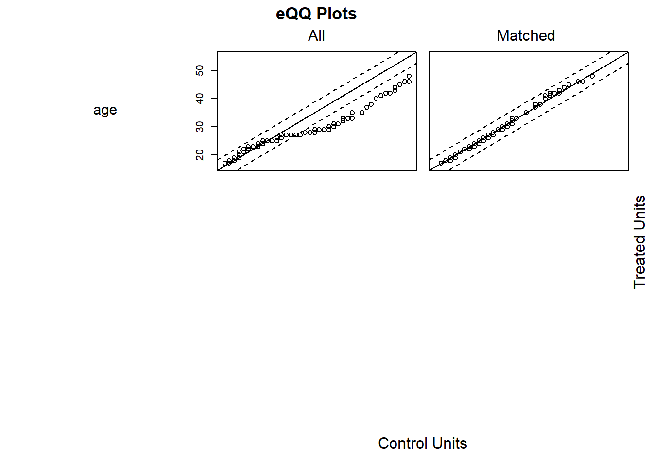
#> - covariates: age, educ- Check balance
Sometimes you have to make trade-off between balance and sample size.
# Checking balance after NN matching
summary(m.out1, un = FALSE)
#>
#> Call:
#> matchit(formula = treat ~ age + educ, data = lalonde, method = "nearest",
#>     distance = "glm")
#>
#> Summary of Balance for Matched Data:
#>          Means Treated Means Control Std. Mean Diff. Var. Ratio eCDF Mean
#> distance        0.3080        0.3077          0.0094     0.9963    0.0033
#> age            25.8162       25.8649         -0.0068     1.0300    0.0050
#> educ           10.3459       10.2865          0.0296     0.5886    0.0253
#>          eCDF Max Std. Pair Dist.
#> distance   0.0432          0.0146
#> age        0.0162          0.0597
#> educ       0.1189          0.8146
#>
#> Sample Sizes:
#>           Control Treated
#> All           429     185
#> Matched       185     185
#> Unmatched     244       0
#> Discarded       0       0

# examine visually
plot(m.out1, type = "jitter", interactive = FALSE)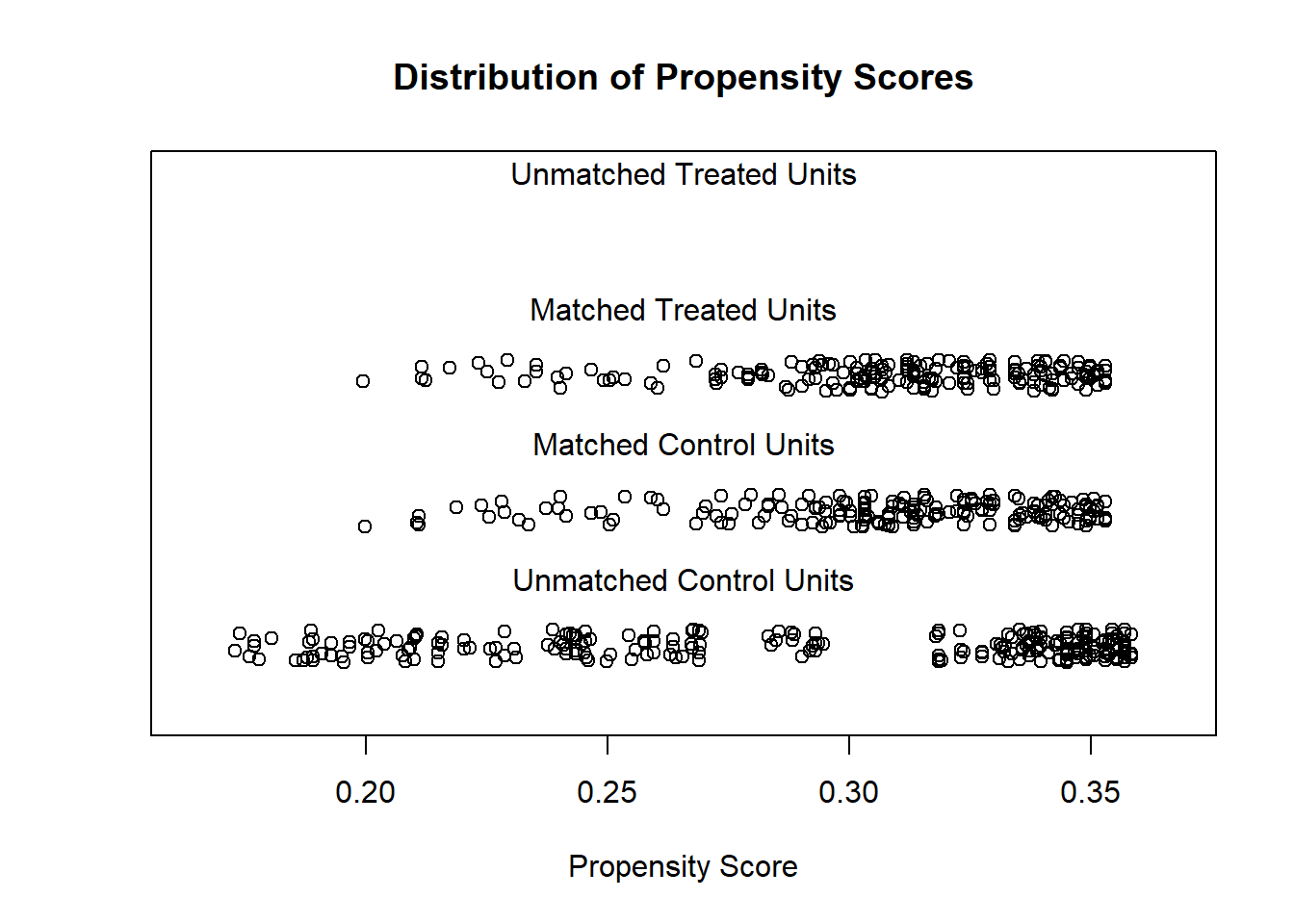
Try Full Match (i.e., every treated matches with one control, and every control with one treated).
# Full matching on a probit PS
m.out2 <- matchit(treat ~ age + educ,
                  data = lalonde,
                  method = "full",
                  distance = "glm",
                  link = "probit")
m.out2
#> A matchit object
#>  - method: Optimal full matching
#>  - distance: Propensity score
#>              - estimated with probit regression
#>  - number of obs.: 614 (original), 614 (matched)
#>  - target estimand: ATT
#>  - covariates: age, educ
Checking balance again
# Checking balance after full matching
summary(m.out2, un = FALSE)
#>
#> Call:
#> matchit(formula = treat ~ age + educ, data = lalonde, method = "full",
#>     distance = "glm", link = "probit")
#>
#> Summary of Balance for Matched Data:
#>          Means Treated Means Control Std. Mean Diff. Var. Ratio eCDF Mean
#> distance        0.3082        0.3081          0.0023     0.9815    0.0028
#> age            25.8162       25.8035          0.0018     0.9825    0.0062
#> educ           10.3459       10.2315          0.0569     0.4390    0.0481
#>          eCDF Max Std. Pair Dist.
#> distance   0.0270          0.0382
#> age        0.0249          0.1110
#> educ       0.1300          0.9805
#>
#> Sample Sizes:
#>               Control Treated
#> All            429.       185
#> Matched (ESS)  145.23     185
#> Matched        429.       185
#> Unmatched        0.         0
#> Discarded        0.         0

plot(summary(m.out2))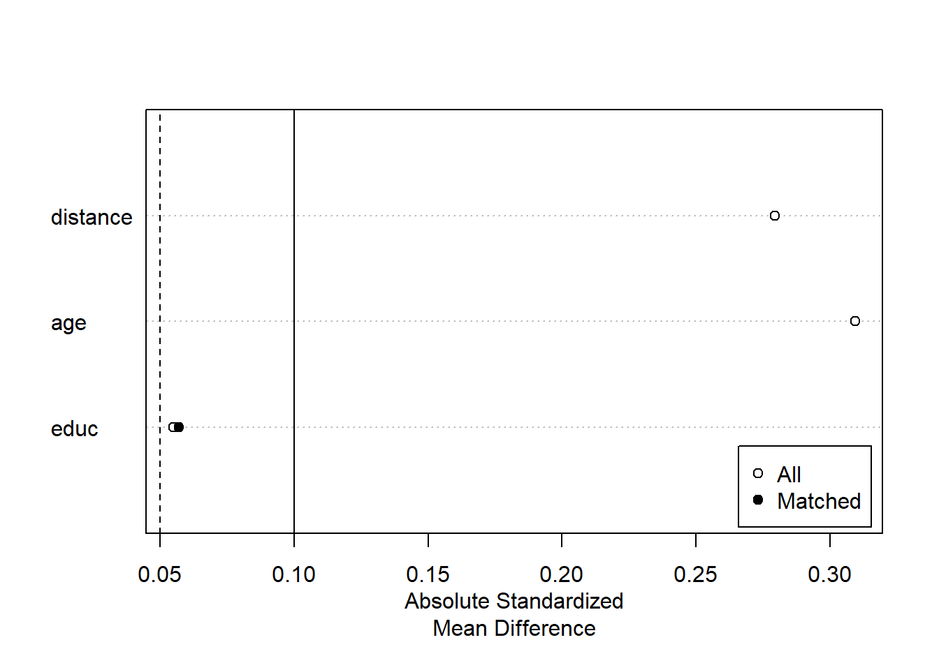
Exact Matching
# Full matching on a probit PS
m.out3 <-
    matchit(
        treat ~ age + educ,
        data = lalonde,
        method = "exact"
    )
m.out3
#> A matchit object
#>  - method: Exact matching
#>  - number of obs.: 614 (original), 332 (matched)
#>  - target estimand: ATT
#>  - covariates: age, educ
Subclassfication
m.out4 <- matchit(
    treat ~ age + educ,
    data = lalonde,
    method = "subclass"
)
m.out4
#> A matchit object
#>  - method: Subclassification (6 subclasses)
#>  - distance: Propensity score
#>              - estimated with logistic regression
#>  - number of obs.: 614 (original), 614 (matched)
#>  - target estimand: ATT
#>  - covariates: age, educ

# Or you can use in conjunction with "nearest"
m.out4 <- matchit(
    treat ~ age + educ,
    data = lalonde,
    method = "nearest",
    option = "subclass"
)
m.out4
#> A matchit object
#>  - method: 1:1 nearest neighbor matching without replacement
#>  - distance: Propensity score
#>              - estimated with logistic regression
#>  - number of obs.: 614 (original), 370 (matched)
#>  - target estimand: ATT
#>  - covariates: age, educ
Optimal Matching
m.out5 <- matchit(
    treat ~ age + educ,
    data = lalonde,
    method = "optimal",
    ratio = 2
)
m.out5
#> A matchit object
#>  - method: 2:1 optimal pair matching
#>  - distance: Propensity score
#>              - estimated with logistic regression
#>  - number of obs.: 614 (original), 555 (matched)
#>  - target estimand: ATT
#>  - covariates: age, educ
Genetic Matching
m.out6 <- matchit(
    treat ~ age + educ,
    data = lalonde,
    method = "genetic"
)
m.out6
#> A matchit object
#>  - method: 1:1 genetic matching without replacement
#>  - distance: Propensity score
#>              - estimated with logistic regression
#>  - number of obs.: 614 (original), 370 (matched)
#>  - target estimand: ATT
#> - covariates: age, educ- Estimating the Treatment Effect
# get matched data
m.data1 <- match.data(m.out1)

head(m.data1)
#>      treat age educ   race married nodegree re74 re75       re78  distance
#> NSW1     1  37   11  black       1        1    0    0  9930.0460 0.2536942
#> NSW2     1  22    9 hispan       0        1    0    0  3595.8940 0.3245468
#> NSW3     1  30   12  black       0        0    0    0 24909.4500 0.2881139
#> NSW4     1  27   11  black       0        1    0    0  7506.1460 0.3016672
#> NSW5     1  33    8  black       0        1    0    0   289.7899 0.2683025
#> NSW6     1  22    9  black       0        1    0    0  4056.4940 0.3245468
#>      weights subclass
#> NSW1       1        1
#> NSW2       1       98
#> NSW3       1      109
#> NSW4       1      120
#> NSW5       1      131
#> NSW6       1      142
library("lmtest") #coeftest
library("sandwich") #vcovCL

# imbalance matched dataset
fit1 <- lm(re78 ~ treat + age + educ ,
           data = m.data1,
           weights = weights)

coeftest(fit1, vcov. = vcovCL, cluster = ~subclass)
#>
#> t test of coefficients:
#>
#>              Estimate Std. Error t value Pr(>|t|)
#> (Intercept)  -174.902   2445.013 -0.0715 0.943012
#> treat       -1139.085    780.399 -1.4596 0.145253
#> age           153.133     55.317  2.7683 0.005922 **
#> educ          358.577    163.860  2.1883 0.029278 *
#> ---
#> Signif. codes:  0 '***' 0.001 '**' 0.01 '*' 0.05 '.' 0.1 ' ' 1
treat coefficient = estimated ATT
# balance matched dataset
m.data2 <- match.data(m.out2)

fit2 <- lm(re78 ~ treat + age + educ ,
           data = m.data2, weights = weights)

coeftest(fit2, vcov. = vcovCL, cluster = ~subclass)
#>
#> t test of coefficients:
#>
#>             Estimate Std. Error t value Pr(>|t|)
#> (Intercept) 2151.952   3141.152  0.6851  0.49355
#> treat       -725.184    703.297 -1.0311  0.30289
#> age          120.260     53.933  2.2298  0.02612 *
#> educ         175.693    241.694  0.7269  0.46755
#> ---
#> Signif. codes:  0 '***' 0.001 '**' 0.01 '*' 0.05 '.' 0.1 ' ' 1
When reporting, remember to mention
- the matching specification (method, and additional options)
- the distance measure (e.g., propensity score)
- other methods, and rationale for the final chosen method.
- balance statistics of the matched dataset.
- number of matched, unmatched, discarded
- estimation method for treatment effect.
31.1.2 designmatch
This package includes
distmatchoptimal distance matchingbmatchoptimal bipartile matchingcardmatchoptimal cardinality matchingprofmatchoptimal profile matchingnmatchoptimal nonbipartile matching
library(designmatch)31.1.3 MatchingFrontier
As mentioned in MatchIt, you have to make trade-off (also known as bias-variance trade-off) between balance and sample size. An automated procedure to optimize this trade-off is implemented in MatchingFrontier (G. King, Lucas, and Nielsen 2017), which solves this joint optimization problem.
Following MatchingFrontier guide
# library(devtools)
# install_github('ChristopherLucas/MatchingFrontier')
library(MatchingFrontier)
data("lalonde")
# choose var to match on
match.on <-
    colnames(lalonde)[!(colnames(lalonde) %in% c('re78', 'treat'))]
match.on

# Mahanlanobis frontier (default)
mahal.frontier <-
    makeFrontier(
        dataset = lalonde,
        treatment = "treat",
        match.on = match.on
    )
mahal.frontier

# L1 frontier
L1.frontier <-
    makeFrontier(
        dataset = lalonde,
        treatment = 'treat',
        match.on = match.on,
        QOI = 'SATT',
        metric = 'L1',
        ratio = 'fixed'
    )
L1.frontier

# estimate effects along the frontier

# Set base form
my.form <-
    as.formula(re78 ~ treat + age + black + education
               + hispanic + married + nodegree + re74 + re75)

# Estimate effects for the mahalanobis frontier
mahal.estimates <-
    estimateEffects(
        mahal.frontier,
        're78 ~ treat',
        mod.dependence.formula = my.form,
        continuous.vars = c('age', 'education', 're74', 're75'),
        prop.estimated = .1,
        means.as.cutpoints = TRUE
    )

# Estimate effects for the L1 frontier
L1.estimates <-
    estimateEffects(
        L1.frontier,
        're78 ~ treat',
        mod.dependence.formula = my.form,
        continuous.vars = c('age', 'education', 're74', 're75'),
        prop.estimated = .1,
        means.as.cutpoints = TRUE
    )

# Plot covariates means
# plotPrunedMeans()


# Plot estimates (deprecated)
# plotEstimates(
#     L1.estimates,
#     ylim = c(-10000, 3000),
#     cex.lab = 1.4,
#     cex.axis = 1.4,
#     panel.first = grid(NULL, NULL, lwd = 2,)
# )

# Plot estimates
plotMeans(L1.frontier)


# parallel plot
parallelPlot(
    L1.frontier,
    N = 400,
    variables = c('age', 're74', 're75', 'black'),
    treated.col = 'blue',
    control.col = 'gray'
)

# export matched dataset
# take 400 units
matched.data <- generateDataset(L1.frontier, N = 400)
31.1.4 Propensity Scores
Even though I mention the propensity scores matching method here, it is no longer recommended to use such method in research and publication (G. King and Nielsen 2019) because it increases
imbalance
inefficiency
model dependence: small changes in the model specification lead to big changes in model results
bias
(Abadie and Imbens 2016)note
The initial estimation of the propensity score influences the large sample distribution of the estimators.
-
Adjustments are made to the large sample variances of these estimators for both ATE and ATT.
The adjustment for the ATE estimator is either negative or zero, indicating greater efficiency when matching on an estimated propensity score versus the true score in large samples.
For the ATET estimator, the sign of the adjustment depends on the data generating process. Neglecting the estimation error in the propensity score can lead to inaccurate confidence intervals for the ATT estimator, making them either too large or too small.
PSM tries to accomplish complete randomization while other methods try to achieve fully blocked. Hence, you probably better off use any other methods.
Propensity is “the probability of receiving the treatment given the observed covariates.” (Rosenbaum and Rubin 1985)
Equivalently, it can to understood as the probability of being treated.
\[ e_i (X_i) = P(T_i = 1 | X_i) \]
Estimation using
logistic regression
-
Non parametric methods:
boosted CART
generalized boosted models (gbm)
Steps by Gary King’s slides
reduce k elements of X to scalar
\(\pi_i \equiv P(T_i = 1|X) = \frac{1}{1+e^{X_i \beta}}\)
Distance (\(X_c, X_t\)) = \(|\pi_c - \pi_t|\)
match each treated unit to the nearest control unit
control units: not reused; pruned if unused
prune matches if distances > caliper
In the best case scenario, you randomly prune, which increases imbalance
Other methods dominate because they try to match exactly hence
\(X_c = X_t \to \pi_c = \pi_t\) (exact match leads to equal propensity scores) but
\(\pi_c = \pi_t \nrightarrow X_c = X_t\) (equal propensity scores do not necessarily lead to exact match)
Notes:
Do not include/control for irrelevant covariates because it leads your PSM to be more random, hence more imbalance
Do not include for (Bhattacharya and Vogt 2007) instrumental variable in the predictor set of a propensity score matching estimator. More generally, using variables that do not control for potential confounders, even if they are predictive of the treatment, can result in biased estimates
What you left with after pruning is more important than what you start with then throw out.
Diagnostics:
balance of the covariates
no need to concern about collinearity
can’t use c-stat or stepwise because those model fit stat do not apply
31.1.5 Mahalanobis Distance
Approximates fully blocked experiment
Distance \((X_c,X_t)\) = \(\sqrt{(X_c - X_t)'S^{-1}(X_c - X_t)}\)
where \(S^{-1}\) standardize the distance
In application we use Euclidean distance.
Prune unused control units, and prune matches if distance > caliper
31.1.6 Coarsened Exact Matching
Steps from Gray King’s slides International Methods Colloquium talk 2015
Temporarily coarsen \(X\)
-
Apply exact matching to the coarsened \(X, C(X)\)
sort observation into strata, each with unique values of \(C(X)\)
prune stratum with 0 treated or 0 control units
Pass on original (uncoarsened) units except those pruned
Properties:
-
Monotonic imbalance bounding (MIB) matching method
- maximum imbalance between the treated and control chosen ex ante
meets congruence principle
robust to measurement error
can be implemented with multiple imputation
works well for multi-category treatments
Assumptions:
- Ignorability (i.e., no omitted variable bias)
More detail in (Iacus, King, and Porro 2012)
Example by package’s authors
library(cem)
data(LeLonde)

Le <- data.frame(na.omit(LeLonde)) # remove missing data
# treated and control groups
tr <- which(Le$treated==1)
ct <- which(Le$treated==0)
ntr <- length(tr)
nct <- length(ct)

# unadjusted, biased difference in means
mean(Le$re78[tr]) - mean(Le$re78[ct])
#> [1] 759.0479

# pre-treatment covariates
vars <-
    c(
        "age",
        "education",
        "black",
        "married",
        "nodegree",
        "re74",
        "re75",
        "hispanic",
        "u74",
        "u75",
        "q1"
    )

# overall imbalance statistics
imbalance(group=Le$treated, data=Le[vars]) # L1 = 0.902
#>
#> Multivariate Imbalance Measure: L1=0.902
#> Percentage of local common support: LCS=5.8%
#>
#> Univariate Imbalance Measures:
#>
#>               statistic   type           L1 min 25%      50%       75%
#> age        -0.252373042 (diff) 5.102041e-03   0   0   0.0000   -1.0000
#> education   0.153634710 (diff) 8.463851e-02   1   0   1.0000    1.0000
#> black      -0.010322734 (diff) 1.032273e-02   0   0   0.0000    0.0000
#> married    -0.009551495 (diff) 9.551495e-03   0   0   0.0000    0.0000
#> nodegree   -0.081217371 (diff) 8.121737e-02   0  -1   0.0000    0.0000
#> re74      -18.160446880 (diff) 5.551115e-17   0   0 284.0715  806.3452
#> re75      101.501761679 (diff) 5.551115e-17   0   0 485.6310 1238.4114
#> hispanic   -0.010144756 (diff) 1.014476e-02   0   0   0.0000    0.0000
#> u74        -0.045582186 (diff) 4.558219e-02   0   0   0.0000    0.0000
#> u75        -0.065555292 (diff) 6.555529e-02   0   0   0.0000    0.0000
#> q1          7.494021189 (Chi2) 1.067078e-01  NA  NA       NA        NA
#>                  max
#> age          -6.0000
#> education     1.0000
#> black         0.0000
#> married       0.0000
#> nodegree      0.0000
#> re74      -2139.0195
#> re75        490.3945
#> hispanic      0.0000
#> u74           0.0000
#> u75           0.0000
#> q1                NA

# drop other variables that are not pre - treatmentt matching variables
todrop <- c("treated", "re78")
imbalance(group=Le$treated, data=Le, drop=todrop)
#>
#> Multivariate Imbalance Measure: L1=0.902
#> Percentage of local common support: LCS=5.8%
#>
#> Univariate Imbalance Measures:
#>
#>               statistic   type           L1 min 25%      50%       75%
#> age        -0.252373042 (diff) 5.102041e-03   0   0   0.0000   -1.0000
#> education   0.153634710 (diff) 8.463851e-02   1   0   1.0000    1.0000
#> black      -0.010322734 (diff) 1.032273e-02   0   0   0.0000    0.0000
#> married    -0.009551495 (diff) 9.551495e-03   0   0   0.0000    0.0000
#> nodegree   -0.081217371 (diff) 8.121737e-02   0  -1   0.0000    0.0000
#> re74      -18.160446880 (diff) 5.551115e-17   0   0 284.0715  806.3452
#> re75      101.501761679 (diff) 5.551115e-17   0   0 485.6310 1238.4114
#> hispanic   -0.010144756 (diff) 1.014476e-02   0   0   0.0000    0.0000
#> u74        -0.045582186 (diff) 4.558219e-02   0   0   0.0000    0.0000
#> u75        -0.065555292 (diff) 6.555529e-02   0   0   0.0000    0.0000
#> q1          7.494021189 (Chi2) 1.067078e-01  NA  NA       NA        NA
#>                  max
#> age          -6.0000
#> education     1.0000
#> black         0.0000
#> married       0.0000
#> nodegree      0.0000
#> re74      -2139.0195
#> re75        490.3945
#> hispanic      0.0000
#> u74           0.0000
#> u75           0.0000
#> q1                NA
automated coarsening
mat <-
    cem(
        treatment = "treated",
        data = Le,
        drop = "re78",
        keep.all = TRUE
    )
#>
#> Using 'treated'='1' as baseline group
mat
#>            G0  G1
#> All       392 258
#> Matched    95  84
#> Unmatched 297 174

# mat$w
coarsening by explicit user choice
# categorial variables
levels(Le$q1) # grouping option
#> [1] "agree"             "disagree"          "neutral"
#> [4] "no opinion"        "strongly agree"    "strongly disagree"
q1.grp <-
    list(
        c("strongly agree", "agree"),
        c("neutral", "no opinion"),
        c("strongly disagree", "disagree")
    ) # if you want ordered categories

# continuous variables
table(Le$education)
#>
#>   3   4   5   6   7   8   9  10  11  12  13  14  15
#>   1   5   4   6  12  55 106 146 173 113  19   9   1
educut <- c(0, 6.5, 8.5, 12.5, 17)  # use cutpoints

mat1 <-
    cem(
        treatment = "treated",
        data = Le,
        drop = "re78",
        cutpoints = list(education = educut),
        grouping = list(q1 = q1.grp)
    )
#>
#> Using 'treated'='1' as baseline group
mat1
#>            G0  G1
#> All       392 258
#> Matched   158 115
#> Unmatched 234 143
Can also use progressive coarsening method to control the number of matches.
cemcan also handle some missingness.
31.1.7 Genetic Matching
-
GM uses iterative checking process of propensity scores, which combines propensity scores and Mahalanobis distance.
- GenMatch (Diamond and Sekhon 2013)
GM is arguably “superior” method than nearest neighbor or full matching in imbalanced data
Use a genetic search algorithm to find weights for each covariate such that we have optimal balance.
-
Implementation
could use with replacement
-
balance can be based on
paired \(t\)-tests (dichotomous variables)
Kolmogorov-Smirnov (multinomial and continuous)
Packages
Matching
library(Matching)
data(lalonde)
attach(lalonde)

#The covariates we want to match on
X = cbind(age, educ, black, hisp, married, nodegr, u74, u75, re75, re74)

#The covariates we want to obtain balance on
BalanceMat <-
    cbind(age,
          educ,
          black,
          hisp,
          married,
          nodegr,
          u74,
          u75,
          re75,
          re74,
          I(re74 * re75))

#
#Let's call GenMatch() to find the optimal weight to give each
#covariate in 'X' so as we have achieved balance on the covariates in
#'BalanceMat'. This is only an example so we want GenMatch to be quick
#so the population size has been set to be only 16 via the 'pop.size'
#option. This is *WAY* too small for actual problems.
#For details see http://sekhon.berkeley.edu/papers/MatchingJSS.pdf.
#
genout <-
    GenMatch(
        Tr = treat,
        X = X,
        BalanceMatrix = BalanceMat,
        estimand = "ATE",
        M = 1,
        pop.size = 16,
        max.generations = 10,
        wait.generations = 1
    )

#The outcome variable
Y=re78/1000

#
# Now that GenMatch() has found the optimal weights, let's estimate
# our causal effect of interest using those weights
#
mout <-
    Match(
        Y = Y,
        Tr = treat,
        X = X,
        estimand = "ATE",
        Weight.matrix = genout
    )
summary(mout)

#
#Let's determine if balance has actually been obtained on the variables of interest
#
mb <-
    MatchBalance(
        treat ~ age + educ + black + hisp + married + nodegr
        + u74 + u75 + re75 + re74 + I(re74 * re75),
        match.out = mout,
        nboots = 500
    )
31.1.8 Entropy Balancing
Entropy balancing is a method for achieving covariate balance in observational studies with binary treatments.
It uses a maximum entropy reweighting scheme to ensure that treatment and control groups are balanced based on sample moments.
This method adjusts for inequalities in the covariate distributions, reducing dependence on the model used for estimating treatment effects.
Entropy balancing improves balance across all included covariate moments and removes the need for repetitive balance checking and iterative model searching.
31.1.9 Matching for high-dimensional data
One could reduce the number of dimensions using methods such as:
Lasso (Gordon et al. 2019)
Penalized logistic regression (Eckles and Bakshy 2021)
PCA (Principal Component Analysis)
Locality Preserving Projections (LPP) (S. Li et al. 2016)
Random projection
Autoencoders (Ramachandra 2018)
Additionally, one could jointly does dimension reduction while balancing the distributions of the control and treated groups (Yao et al. 2018).
31.1.10 Matching for time series-cross-section data
Examples: (Scheve and Stasavage 2012) and (Acemoglu et al. 2019)
Identification strategy:
Within-unit over-time variation
within-time across-units variation
See DID with in and out treatment condition for details of this method
31.1.11 Matching for multiple treatments
In cases where you have multiple treatment groups, and you want to do matching, it’s important to have the same baseline (control) group. For more details, see
(Zhao et al. 2021): also for continuous treatment
If you insist on using the MatchIt package, then see this answer
31.1.12 Matching for multi-level treatments
See (Yang et al. 2016)
Package in R shuyang1987/multilevelMatching on Github
31.1.13 Matching for repeated treatments
https://cran.r-project.org/web/packages/twang/vignettes/iptw.pdf
package in R twang
31.2 Selection on Unobservables
There are several ways one can deal with selection on unobservables:
Endogenous Sample Selection (i.e., Heckman-style correction): examine the \(\lambda\) term to see whether it’s significant (sign of endogenous selection)
31.2.1 Rosenbaum Bounds
Examples in marketing
(Oestreicher-Singer and Zalmanson 2013): A range of 1.5 to 1.8 is important for the effect of the level of community participation of users on their willingness to pay for premium services.
(M. Sun and Zhu 2013): A factor of 1.5 is essential for understanding the relationship between the launch of an ad revenue-sharing program and the popularity of content.
(Manchanda, Packard, and Pattabhiramaiah 2015): A factor of 1.6 is required for the social dollar effect to be nullified.
(Sudhir and Talukdar 2015): A factor of 1.9 is needed for IT adoption to impact labor productivity, and 2.2 for IT adoption to affect floor productivity.
(Proserpio and Zervas 2017b): A factor of 2 is necessary for the firm’s use of management responses to influence online reputation.
(S. Zhang et al. 2022): A factor of 1.55 is critical for the acquisition of verified images to drive demand for Airbnb properties.
(Chae, Ha, and Schweidel 2023): A factor of 27 (not a typo) is significant in how paywall suspensions affect subsequent subscription decisions.
General
-
Matching Methods are favored for estimating treatment effects in observational data, offering advantages over regression methods because
It reduces reliance on functional form assumptions.
Assumes all selection-influencing covariates are observable; estimates are unbiased if no unobserved confounders are missed.
-
Concerns arise when potentially relevant covariates are unmeasured.
- Rosenbaum Bounds assess the overall sensitivity of coefficient estimates to hidden bias (Rosenbaum and Rosenbaum 2002) without having knowledge (e.g., direction) of the bias. Because the unboservables that cause hidden bias have to both affect selection into treatment by a factor of \(\Gamma\) and predictive of outcome, this method is also known as worst case analyses (DiPrete and Gangl 2004).
Can’t provide precise bounds on estimates of treatment effects (see Relative Correlation Restrictions)
Typically, we show both p-value and H-L point estimate for each level of gamma \(\Gamma\)
With random treatment assignment, we can use the non-parametric test (Wilcoxon signed rank test) to see if there is treatment effect.
Without random treatment assignment (i.e., observational data), we cannot use this test. With Selection on Observables, we can use this test if we believe there are no unmeasured confounders. And this is where Rosenbaum (2002) can come in to talk about the believability of this notion.
In layman’s terms, consider that the treatment assignment is based on a method where the odds of treatment for a unit and its control differ by a multiplier \(\Gamma\)
- For example, \(\Gamma = 1\) means that the odds of assignment are identical, indicating random treatment assignment.
- Another example, \(\Gamma = 2\), in the same matched pair, one unit is twice as likely to receive the treatment (due to unobservables).
- Since we can’t know \(\Gamma\) with certainty, we run sensitivity analysis to see if the results change with different values of \(\Gamma\)
- This bias is the product of an unobservable that influences both treatment selection and outcome by a factor \(\Gamma\) (omitted variable bias)
In technical terms,
-
Treatment Assignment and Probability:
- Consider unit \(j\) with a probability \(\pi_j\) of receiving the treatment, and unit \(i\) with \(\pi_i\).
- Ideally, after matching, if there’s no hidden bias, we’d have \(\pi_i = \pi_j\).
- However, observing \(\pi_i \neq \pi_j\) raises questions about potential biases affecting our inference. This is evaluated using the odds ratio.
-
Odds Ratio and Hidden Bias:
- The odds of treatment for a unit \(j\) is defined as \(\frac{\pi_j}{1 - \pi_j}\).
- The odds ratio between two matched units \(i\) and \(j\) is constrained by \(\frac{1}{\Gamma} \le \frac{\pi_i / (1- \pi_i)}{\pi_j/ (1- \pi_j)} \le \Gamma\).
- If \(\Gamma = 1\), it implies an absence of hidden bias.
- If \(\Gamma = 2\), the odds of receiving treatment could differ by up to a factor of 2 between the two units.
-
Sensitivity Analysis Using Gamma:
- The value of \(\Gamma\) helps measure the potential departure from a bias-free study.
- Sensitivity analysis involves varying \(\Gamma\) to examine how inferences might change with the presence of hidden biases.
-
Incorporating Unobserved Covariates:
- Consider a scenario where unit \(i\) has observed covariates \(x_i\) and an unobserved covariate \(u_i\), that both affect the outcome.
- A logistic regression model could link the odds of assignment to these covariates: \(\log(\frac{\pi_i}{1 - \pi_i}) = \kappa x_i + \gamma u_i\), where \(\gamma\) represents the impact of the unobserved covariate.
-
Steps for Sensitivity Analysis (We could create a table of different levels of \(\Gamma\) to assess how the magnitude of biases can affect our evidence of the treatment effect (estimate):
- Select a range of values for \(\Gamma\) (e.g., \(1 \to 2\)).
- Assess how the p-value or the magnitude of the treatment effect (Hodges Jr and Lehmann 2011) (for more details, see (Hollander, Wolfe, and Chicken 2013)) changes with varying \(\Gamma\) values.
- Employ specific randomization tests based on the type of outcome to establish bounds on inferences.
- report the minimum value of \(\Gamma\) at which the treatment treat is nullified (i.e., become insignificant). And the literature’s rules of thumb is that if \(\Gamma > 2\), then we have strong evidence for our treatment effect is robust to large biases (Proserpio and Zervas 2017a)
Notes:
- If we have treatment assignment is clustered (e.g., within school, within state) we need to adjust the bounds for clustered treatment assignment (B. B. Hansen, Rosenbaum, and Small 2014) (similar to clustered standard errors).
Packages
rbounds(Keele 2010)sensitivitymv(Rosenbaum 2015)
Since we typically assess our estimate sensitivity to unboservables after matching, we first do some matching.
library(MatchIt)
library(Matching)
data("lalonde")

matched <- MatchIt::matchit(
    treat ~ age + educ,
    data = lalonde,
    method = "nearest"
)
summary(matched)
#>
#> Call:
#> MatchIt::matchit(formula = treat ~ age + educ, data = lalonde,
#>     method = "nearest")
#>
#> Summary of Balance for All Data:
#>          Means Treated Means Control Std. Mean Diff. Var. Ratio eCDF Mean
#> distance        0.4203        0.4125          0.1689     1.2900    0.0431
#> age            25.8162       25.0538          0.1066     1.0278    0.0254
#> educ           10.3459       10.0885          0.1281     1.5513    0.0287
#>          eCDF Max
#> distance   0.1251
#> age        0.0652
#> educ       0.1265
#>
#> Summary of Balance for Matched Data:
#>          Means Treated Means Control Std. Mean Diff. Var. Ratio eCDF Mean
#> distance        0.4203        0.4179          0.0520     1.1691    0.0105
#> age            25.8162       25.5081          0.0431     1.1518    0.0148
#> educ           10.3459       10.2811          0.0323     1.5138    0.0224
#>          eCDF Max Std. Pair Dist.
#> distance   0.0595          0.0598
#> age        0.0486          0.5628
#> educ       0.0757          0.3602
#>
#> Sample Sizes:
#>           Control Treated
#> All           260     185
#> Matched       185     185
#> Unmatched      75       0
#> Discarded       0       0
matched_data <- match.data(matched)

treatment_group <- subset(matched_data, treat == 1)
control_group <- subset(matched_data, treat == 0)


library(rbounds)

# p-value sensitivity
psens_res <-
    psens(treatment_group$re78,
          control_group$re78,
          Gamma = 2,
          GammaInc = .1)

psens_res
#>
#>  Rosenbaum Sensitivity Test for Wilcoxon Signed Rank P-Value
#>
#> Unconfounded estimate ....  0.0058
#>
#>  Gamma Lower bound Upper bound
#>    1.0      0.0058      0.0058
#>    1.1      0.0011      0.0235
#>    1.2      0.0002      0.0668
#>    1.3      0.0000      0.1458
#>    1.4      0.0000      0.2599
#>    1.5      0.0000      0.3967
#>    1.6      0.0000      0.5378
#>    1.7      0.0000      0.6664
#>    1.8      0.0000      0.7723
#>    1.9      0.0000      0.8523
#>    2.0      0.0000      0.9085
#>
#>  Note: Gamma is Odds of Differential Assignment To
#>  Treatment Due to Unobserved Factors
#>

# Hodges-Lehmann point estimate sensitivity
# median difference between treatment and control
hlsens_res <-
    hlsens(treatment_group$re78,
           control_group$re78,
           Gamma = 2,
           GammaInc = .1)
hlsens_res
#>
#>  Rosenbaum Sensitivity Test for Hodges-Lehmann Point Estimate
#>
#> Unconfounded estimate ....  1745.843
#>
#>  Gamma Lower bound Upper bound
#>    1.0 1745.800000      1745.8
#>    1.1 1139.100000      1865.6
#>    1.2  830.840000      2160.9
#>    1.3  533.740000      2462.4
#>    1.4  259.940000      2793.8
#>    1.5   -0.056912      3059.3
#>    1.6 -144.960000      3297.8
#>    1.7 -380.560000      3535.7
#>    1.8 -554.360000      3751.0
#>    1.9 -716.360000      4012.1
#>    2.0 -918.760000      4224.3
#>
#>  Note: Gamma is Odds of Differential Assignment To
#>  Treatment Due to Unobserved Factors
#>
For multiple control group matching
library(Matching)
library(MatchIt)

n_ratio <- 2
matched <- MatchIt::matchit(treat ~ age + educ ,
                   method = "nearest", ratio = n_ratio)
summary(matched)
matched_data <- match.data(matched)

mcontrol_res <- rbounds::mcontrol(
    y          = matched_data$re78,
    grp.id     = matched_data$subclass,
    treat.id   = matched_data$treat,
    group.size = n_ratio + 1,
    Gamma      = 2.5,
    GammaInc   = .1
)

mcontrol_res
sensitivitymw is faster than sensitivitymw. But sensitivitymw can match where matched sets can have differing numbers of controls (Rosenbaum 2015).
library(sensitivitymv)
data(lead150)
head(lead150)
#> [,1] [,2] [,3] [,4] [,5] [,6]
#> [1,] 1.40 1.23 2.24 0.96 1.90 1.14
#> [2,] 0.63 0.99 0.87 1.90 0.67 1.40
#> [3,] 1.98 0.82 0.66 0.58 1.00 1.30
#> [4,] 1.45 0.53 1.43 1.70 0.85 1.50
#> [5,] 1.60 1.70 0.63 1.05 1.08 0.92
#> [6,] 1.13 0.31 0.71 1.10 0.86 1.14
senmv(lead150,gamma=2,trim=2)
#> $pval
#> [1] 0.02665519
#>
#> $deviate
#> [1] 1.932398
#>
#> $statistic
#> [1] 27.97564
#>
#> $expectation
#> [1] 18.0064
#>
#> $variance
#> [1] 26.61524
library(sensitivitymw)
senmw(lead150,gamma=2,trim=2)
#> $pval
#> [1] 0.02665519
#>
#> $deviate
#> [1] 1.932398
#>
#> $statistic
#> [1] 27.97564
#>
#> $expectation
#> [1] 18.0064
#>
#> $variance
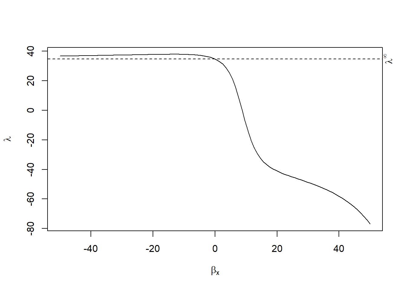
#> [1] 26.6152431.2.2 Relative Correlation Restrictions
Examples in marketing
(Manchanda, Packard, and Pattabhiramaiah 2015): 3.23 for social dollar effect to be nullified
(Chae, Ha, and Schweidel 2023): 6.69 (i.e., how much stronger the selection on unobservables has to be compared to the selection on observables to negate the result) for paywall suspensions affect subsequent subscription decisions
General
Proposed by Altonji, Elder, and Taber (2005)
Generalized by Krauth (2016)
Estimate bounds of the treatment effects due to unobserved selection.
\[ Y_i = X_i \beta + C_i \gamma + \epsilon_i \]
where
\(\beta\) is the effect of interest
\(C_i\) is the control variable
Using OLS, \(cor(X_i, \epsilon_i) = 0\)
Under RCR analysis, we assume
\[ cor(X_i, \epsilon_i) = \lambda cor(X_i, C_i \gamma) \]
where \(\lambda \in (\lambda_l, \lambda_h)\)
Choice of \(\lambda\)
Strong assumption of no omitted variable bias (small
If \(\lambda = 0\), then \(cor(X_i, \epsilon_i) = 0\)
If \(\lambda = 1\), then \(cor(X_i, \epsilon_i) = cor(X_i, C_i \gamma)\)
We typically examine \(\lambda \in (0, 1)\)
# remotes::install_github("bvkrauth/rcr/r/rcrbounds")
library(rcrbounds)
# rcrbounds::install_rcrpy()
data("ChickWeight")

rcr_res <-
    rcrbounds::rcr(weight ~ Time |
                       Diet, ChickWeight, rc_range = c(0, 10))
rcr_res
#>
#> Call:
#> rcrbounds::rcr(formula = weight ~ Time | Diet, data = ChickWeight,
#>     rc_range = c(0, 10))
#>
#> Coefficients:
#>     rcInf effectInf       rc0   effectL   effectH
#> 34.676505 71.989336 34.741955  7.447713  8.750492
summary(rcr_res)
#>
#> Call:
#> rcrbounds::rcr(formula = weight ~ Time | Diet, data = ChickWeight,
#>     rc_range = c(0, 10))
#>
#> Coefficients:
#>            Estimate  Std. Error    t value      Pr(>|t|)
#> rcInf     34.676505  50.1295005  0.6917385  4.891016e-01
#> effectInf 71.989336 112.5711682  0.6395007  5.224973e-01
#> rc0       34.741955  58.7169195  0.5916856  5.540611e-01
#> effectL    7.447713   2.4276246  3.0679014  2.155677e-03
#> effectH    8.750492   0.2607671 33.5567355 7.180405e-247
#> ---
#> conservative confidence interval:
#>          2.5  %  97.5  %
#> effect 2.689656 9.261586

# hypothesis test for the coefficient
rcrbounds::effect_test(rcr_res, h0 = 0)
#> [1] 0.001234233
plot(rcr_res)