8 Linear Mixed Models

8.1 Dependent Data

Forms of dependent data:

• Multivariate measurements on different individuals: (e.g., a person’s blood pressure, fat, etc are correlated)
• Clustered measurements: (e.g., blood pressure measurements of people in the same family can be correlated).
• Repeated measurements: (e.g., measurement of cholesterol over time can be correlated) “If data are collected repeatedly on experimental material to which treatments were applied initially, the data is a repeated measure.” (Schabenberger and Pierce 2001)
• Longitudinal data: (e.g., individual’s cholesterol tracked over time are correlated): “data collected repeatedly over time in an observational study are termed longitudinal.” (Schabenberger and Pierce 2001)
• Spatial data: (e.g., measurement of individuals living in the same neighborhood are correlated)

Hence, we like to account for these correlations.

Linear Mixed Model (LMM), also known as Mixed Linear Model has 2 components:

• Fixed effect (e.g, gender, age, diet, time)

• Random effects representing individual variation or auto correlation/spatial effects that imply dependent (correlated) errors

Review Two-Way Mixed Effects ANOVA

We choose to model the random subject-specific effect instead of including dummy subject covariates in our model because:

• reduction in the number of parameters to estimate
• when you do inference, it would make more sense that you can infer from a population (i.e., random effect).

LLM Motivation

In a repeated measurements analysis where \(Y_{ij}\) is the response for the \(i\)-th individual measured at the \(j\)-th time,

\(i =1,…,N\) ; \(j = 1,…,n_i\)

\[ \mathbf{Y}_i = \left( \begin{array} {c} Y_{i1} \\ . \\ .\\ .\\ Y_{in_i} \end{array} \right) \]

is all measurements for subject \(i\).

Stage 1: (Regression Model) how the response changes over time for the \(i\)-th subject

\[ \mathbf{Y_i = Z_i \beta_i + \epsilon_i} \]

where

• \(Z_i\) is an \(n_i \times q\) matrix of known covariates
• \(\beta_i\) is an unknown \(q \times 1\) vector of subjective -specific coefficients (regression coefficients different for each subject)
• \(\epsilon_i\) are the random errors (typically \(\sim N(0, \sigma^2 I)\))

We notice that there are two many \(\beta\) to estimate here. Hence, this is the motivation for the second stage

Stage 2: (Parameter Model)

\[ \mathbf{\beta_i = K_i \beta + b_i} \]

where

• \(K_i\) is a \(q \times p\) matrix of known covariates
• \(\beta\) is a \(p \times 1\) vector of unknown parameter
• \(\mathbf{b}_i\) are independent \(N(0,D)\) random variables

This model explain the observed variability between subjects with respect to the subject-specific regression coefficients, \(\beta_i\). We model our different coefficient (\(\beta_i\)) with respect to \(\beta\).

Example:

Stage 1:

\[ Y_{ij} = \beta_{1i} + \beta_{2i}t_{ij} + \epsilon_{ij} \]

where

• \(j = 1,..,n_i\)

In the matrix notation,

\[ \mathbf{Y_i} = \left( \begin{array} {c} Y_{i1} \\ .\\ Y_{in_i} \end{array} \right); \mathbf{Z}_i = \left( \begin{array} {cc} 1 & t_{i1} \\ . & . \\ 1 & t_{in_i} \end{array} \right) \]

\[ \beta_i = \left( \begin{array} {c} \beta_{1i} \\ \beta_{2i} \end{array} \right); \epsilon_i = \left( \begin{array} {c} \epsilon_{i1} \\ . \\ \epsilon_{in_i} \end{array} \right) \]

Thus,

\[ \mathbf{Y_i = Z_i \beta_i + \epsilon_i} \]

Stage 2:

\[ \begin{aligned} \beta_{1i} &= \beta_0 + b_{1i} \\ \beta_{2i} &= \beta_1 L_i + \beta_2 H_i + \beta_3 C_i + b_{2i} \end{aligned} \]

where \(L_i, H_i, C_i\) are indicator variables defined to 1 as the subject falls into different categories.

Subject specific intercepts do not depend upon treatment, with \(\beta_0\) (the average response at the start of treatment), and \(\beta_1 , \beta_2, \beta_3\) (the average time effects for each of three treatment groups).

\[ \begin{aligned} \mathbf{K}_i &= \left( \begin{array} {cccc} 1 & 0 & 0 & 0 \\ 0 & L_i & H_i & C_i \end{array} \right) \\ \beta &= (\beta_0 , \beta_1, \beta_2, \beta_3)' \\ \mathbf{b}_i &= \left( \begin{array} {c} b_{1i} \\ b_{2i} \\ \end{array} \right) \\ \beta_i &= \mathbf{K_i \beta + b_i} \end{aligned} \]

To get \(\hat{\beta}\), we can fit the model sequentially:

1. Estimate \(\hat{\beta_i}\) in the first stage
2. Estimate \(\hat{\beta}\) in the second stage by replacing \(\beta_i\) with \(\hat{\beta}_i\)

However, problems arise from this method:

• information is lost by summarizing the vector \(\mathbf{Y}_i\) solely by \(\hat{\beta}_i\)
• we need to account for variability when replacing \(\beta_i\) with its estimate
• different subjects might have different number of observations.

To address these problems, we can use Linear Mixed Model (Laird and Ware 1982)

Substituting stage 2 into stage 1:

\[ \mathbf{Y}_i = \mathbf{Z}_i \mathbf{K}_i \beta + \mathbf{Z}_i \mathbf{b}_i + \mathbf{\epsilon}_i \]

Let \(\mathbf{X}_i = \mathbf{Z}_i \mathbf{K}_i\) be an \(n_i \times p\) matrix . Then, the LMM is

\[ \mathbf{Y}_i = \mathbf{X}_i \beta + \mathbf{Z}_i \mathbf{b}_i + \mathbf{\epsilon}_i \]

where

• \(i = 1,..,N\)
• \(\beta\) are the fixed effects, which are common to all subjects
• \(\mathbf{b}_i\) are the subject specific random effects. \(\mathbf{b}_i \sim N_q (\mathbf{0,D})\)
• \(\mathbf{\epsilon}_i \sim N_{n_i}(\mathbf{0,\Sigma_i})\)
• \(\mathbf{b}_i\) and \(\epsilon_i\) are independent
• \(\mathbf{Z}_{i(n_i \times q})\) and \(\mathbf{X}_{i(n_i \times p})\) are matrices of known covariates.

Equivalently, in the hierarchical form, we call conditional or hierarchical formulation of the linear mixed model

\[ \begin{aligned} \mathbf{Y}_i | \mathbf{b}_i &\sim N(\mathbf{X}_i \beta+ \mathbf{Z}_i \mathbf{b}_i, \mathbf{\Sigma}_i) \\ \mathbf{b}_i &\sim N(\mathbf{0,D}) \end{aligned} \]

for \(i = 1,..,N\). denote the respective functions by \(f(\mathbf{Y}_i |\mathbf{b}_i)\) and \(f(\mathbf{b}_i)\)

In general,

\[ \begin{aligned} f(A,B) &= f(A|B)f(B) \\ f(A) &= \int f(A,B)dB = \int f(A|B) f(B) dB \end{aligned} \]

In the LMM, the marginal density of \(\mathbf{Y}_i\) is

\[ f(\mathbf{Y}_i) = \int f(\mathbf{Y}_i | \mathbf{b}_i) f(\mathbf{b}_i) d\mathbf{b}_i \]

which can be shown

\[ \mathbf{Y}_i \sim N(\mathbf{X_i \beta, Z_i DZ'_i + \Sigma_i}) \]

This is the marginal formulation of the linear mixed model

Notes:

We no longer have \(Z_i b_i\) in the mean, but add error in the variance (marginal dependence in Y). kinda of averaging out the common effect. Technically, we shouldn’t call it averaging the error b (adding it to the variance covariance matrix), it should be called adding random effect

Continue with our example

\[ Y_{ij} = (\beta_0 + b_{1i}) + (\beta_1L_i + \beta_2 H_i + \beta_3 C_i + b_{2i})t_{ij} + \epsilon_{ij} \]

for each treatment group

\[ Y_{ik}= \begin{cases} \beta_0 + b_{1i} + (\beta_1 + \ b_{2i})t_{ij} + \epsilon_{ij} & L \\ \beta_0 + b_{1i} + (\beta_2 + \ b_{2i})t_{ij} + \epsilon_{ij} & H\\ \beta_0 + b_{1i} + (\beta_3 + \ b_{2i})t_{ij} + \epsilon_{ij} & C \end{cases} \]

• Intercepts and slopes are all subject specific
• Different treatment groups have different slops, but the same intercept.

In the hierarchical model form

\[ \begin{aligned} \mathbf{Y}_i | \mathbf{b}_i &\sim N(\mathbf{X}_i \beta + \mathbf{Z}_i \mathbf{b}_i, \mathbf{\Sigma}_i)\\ \mathbf{b}_i &\sim N(\mathbf{0,D}) \end{aligned} \]

X will be in the form of

\[ \beta = (\beta_0, \beta_1, \beta_2, \beta_3)' \]

\[ \begin{aligned} \mathbf{X}_i &= \mathbf{Z}_i \mathbf{K}_i \\ &= \left[ \begin{array} {cc} 1 & t_{i1} \\ 1 & t_{i2} \\ . & . \\ 1 & t_{in_i} \end{array} \right] \times \left[ \begin{array} {cccc} 1 & 0 & 0 & 0 \\ 0 & L_i & H_i & C_i \\ \end{array} \right] \\ &= \left[ \begin{array} {cccc} 1 & t_{i1}L_i & t_{i1}H_i & T_{i1}C_i \\ 1 & t_{i2}L_i & t_{i2}H_i & T_{i2}C_i \\ . &. &. &. \\ 1 & t_{in_i}L_i & t_{in_i}H_i & T_{in_i}C_i \\ \end{array} \right]\end{aligned} \]

\[ \mathbf{b}_i = \left( \begin{array} {c} b_{1i} \\ b_{2i} \end{array} \right) \]

\[ D = \left( \begin{array} {cc} d_{11} & d_{12}\\ d_{12} & d_{22} \end{array} \right) \]

Assuming \(\mathbf{\Sigma}_i = \sigma^2 \mathbf{I}_{n_i}\), which is called conditional independence, meaning the response on subject i are independent conditional on \(\mathbf{b}_i\) and \(\beta\)

In the marginal model form

\[ Y_{ij} = \beta_0 + \beta_1 L_i t_{ij} + \beta_2 H_i t_{ij} + \beta_3 C_i t_{ij} + \eta_{ij} \]

where \(\eta_i \sim N(\mathbf{0},\mathbf{Z}_i\mathbf{DZ}_i'+ \mathbf{\Sigma}_i)\)

Equivalently,

\[ \mathbf{Y_i \sim N(X_i \beta, Z_i DZ_i' + \Sigma_i}) \]

In this case that \(n_i = 2\)

\[ \begin{aligned} \mathbf{Z_iDZ_i'} &= \left( \begin{array} {cc} 1 & t_{i1} \\ 1 & t_{i2} \end{array} \right) \left( \begin{array} {cc} d_{11} & d_{12} \\ d_{12} & d_{22} \end{array} \right) \left( \begin{array} {cc} 1 & 1 \\ t_{i1} & t_{i2} \end{array} \right) \\ &= \left( \begin{array} {cc} d_{11} + 2d_{12}t_{i1} + d_{22}t_{i1}^2 & d_{11} + d_{12}(t_{i1} + t_{i2}) + d_{22}t_{i1}t_{i2} \\ d_{11} + d_{12}(t_{i1} + t_{i2}) + d_{22} t_{i1} t_{i2} & d_{11} + 2d_{12}t_{i2} + d_{22}t_{i2}^2 \end{array} \right) \end{aligned} \]

\[ var(Y_{i1}) = d_{11} + 2d_{12}t_{i1} + d_{22} t_{i1}^2 + \sigma^2 \]

On top of correlation in the errors, the marginal implies that the variance function of the response is quadratic over time, with positive curvature \(d_{22}\)

8.1.1 Random-Intercepts Model

If we remove the random slopes,

• the assumption is that all variability in subject-specific slopes can be attributed to treatment differences
• the model is random-intercepts model. This has subject specific intercepts, but the same slopes within each treatment group.

\[ \begin{aligned} \mathbf{Y}_i | b_i &\sim N(\mathbf{X}_i \beta + 1 b_i , \Sigma_i) \\ b_i &\sim N(0,d_{11}) \end{aligned} \]

The marginal model is then (\(\mathbf{\Sigma}_i = \sigma^2 \mathbf{I}\))

\[ \mathbf{Y}_i \sim N(\mathbf{X}_i \beta, 11'd_{11} + \sigma^2 \mathbf{I}) \]

The marginal covariance matrix is

\[ \begin{aligned} cov(\mathbf{Y}_i) &= 11'd_{11} + \sigma^2I \\ &= \left( \begin{array} {cccc} d_{11}+ \sigma^2 & d_{11} & ... & d_{11} \\ d_{11} & d_{11} + \sigma^2 & d_{11} & ... \\ . & . & . & . \\ d_{11} & ... & ... & d_{11} + \sigma^2 \end{array} \right) \end{aligned} \]

the associated correlation matrix is

\[ corr(\mathbf{Y}_i) = \left( \begin{array} {cccc} 1 & \rho & ... & \rho \\ \rho & 1 & \rho & ... \\ . & . & . & . \\ \rho & ... & ... & 1 \\ \end{array} \right) \]

where \(\rho \equiv \frac{d_{11}}{d_{11} + \sigma^2}\)

Thu, we have

• constant variance over time
• equal, positive correlation between any two measurements from the same subject
• a covariance structure that is called compound symmetry, and \(\rho\) is called the intra-class correlation
• that when \(\rho\) is large, the inter-subject variability (\(d_{11}\)) is large relative to the intra-subject variability (\(\sigma^2\))

8.1.2 Covariance Models

If the conditional independence assumption, (\(\mathbf{\Sigma_i= \sigma^2 I_{n_i}}\)). Consider, \(\epsilon_i = \epsilon_{(1)i} + \epsilon_{(2)i}\), where

• \(\epsilon_{(1)i}\) is a “serial correlation” component. That is, part of the individual’s profile is a response to time-varying stochastic processes.
• \(\epsilon_{(2)i}\) is the measurement error component, and is independent of \(\epsilon_{(1)i}\)

Then

\[ \mathbf{Y_i = X_i \beta + Z_i b_i + \epsilon_{(1)i} + \epsilon_{(2)i}} \]

where

• \(\mathbf{b_i} \sim N(\mathbf{0,D})\)

• \(\epsilon_{(2)i} \sim N(\mathbf{0,\sigma^2 I_{n_i}})\)

• \(\epsilon_{(1)i} \sim N(\mathbf{0,\tau^2H_i})\)

• \(\mathbf{b}_i\) and \(\epsilon_i\) are mutually independent

To model the structure of the \(n_i \times n_i\) correlation (or covariance ) matrix \(\mathbf{H}_i\). Let the (j,k)th element of \(\mathbf{H}_i\) be \(h_{ijk}= g(t_{ij}t_{ik})\). that is a function of the times \(t_{ij}\) and \(t_{ik}\) , which is assumed to be some function of the “distance’ between the times.

\[ h_{ijk} = g(|t_{ij}-t_{ik}|) \]

for some decreasing function \(g(.)\) with \(g(0)=1\) (for correlation matrices).

Examples of this type of function:

• Exponential function: \(g(|t_{ij}-t_{ik}|) = \exp(-\phi|t_{ij} - t_{ik}|)\)
• Gaussian function: \(g(|t_{ij} - t_{ik}|) = \exp(-\phi(t_{ij} - t_{ik})^2)\)

Similar structures could also be used for \(\mathbf{D}\) matrix (of \(\mathbf{b}\))

Example: Autoregressive Covariance Structure

A first order Autoregressive Model (AR(1)) has the form

\[ \alpha_t = \phi \alpha_{t-1} + \eta_t \]

where \(\eta_t \sim iid N (0,\sigma^2_\eta)\)

Then, the covariance between two observations is

\[ cov(\alpha_t, \alpha_{t+h}) = \frac{\sigma^2_\eta \phi^{|h|}}{1- \phi^2} \]

for \(h = 0, \pm 1, \pm 2, ...; |\phi|<1\)

Hence,

\[ corr(\alpha_t, \alpha_{t+h}) = \phi^{|h|} \]

If we let \(\alpha_T = (\alpha_1,...\alpha_T)'\), then

\[ corr(\alpha_T) = \left[ \begin{array} {ccccc} 1 & \phi^1 & \phi^2 & ... & \phi^2 \\ \phi^1 & 1 & \phi^1 & ... & \phi^{T-1} \\ \phi^2 & \phi^1 & 1 & ... & \phi^{T-2} \\ . & . & . & . &. \\ \phi^T & \phi^{T-1} & \phi^{T-2} & ... & 1 \end{array} \right] \]

Notes:

• The correlation decreases as time lag increases
• This matrix structure is known as a Toeplitz structure
• More complicated covariance structures are possible, which is critical component of spatial random effects models and time series models.
• Often, we don’t need both random effects \(\mathbf{b}\) and \(\epsilon_{(1)i}\)

More in the Time Series section

8.2 Estimation

\[ \mathbf{Y}_i = \mathbf{X}_i \beta + \mathbf{Z}_i \mathbf{b}_i + \epsilon_i \]

where \(\beta, \mathbf{b}_i, \mathbf{D}, \mathbf{\Sigma}_i\) we must obtain estimation from the data

• \(\mathbf{\beta}, \mathbf{D}, \mathbf{\Sigma}_i\) are unknown, but fixed, parameters, and must be estimated from the data
• \(\mathbf{b}_i\) is a random variable. Thus, we can’t estimate these values, but we can predict them. (i.e., you can’t estimate a random thing).

If we have

• \(\hat{\beta}\) as an estimator of \(\beta\)
• \(\hat{\mathbf{b}}_i\) as a predictor of \(\mathbf{b}_i\)

Then,

• The population average estimate of \(\mathbf{Y}_i\) is \(\hat{\mathbf{Y}_i} = \mathbf{X}_i \hat{\beta}\)
• The subject-specific prediction is \(\hat{\mathbf{Y}_i} = \mathbf{X}_i \hat{\beta} + \mathbf{Z}_i \hat{b}_i\)

According to (Henderson 1975), estimating equations known as the mixed model equations:

\[ \left[ \begin{array} {c} \hat{\beta} \\ \hat{\mathbf{b}} \end{array} \right] = \left[ \begin{array} {cc} \mathbf{X'\Sigma^{-1}X} & \mathbf{X'\Sigma^{-1}Z} \\ \mathbf{Z'\Sigma^{-1}X} & \mathbf{Z'\Sigma^{-1}Z +B^{-1}} \end{array} \right] \left[ \begin{array} {cc} \mathbf{X'\Sigma^{-1}Y} \\ \mathbf{Z'\Sigma^{-1}Y} \end{array} \right] \]

where

\[ \begin{aligned} \mathbf{Y} &= \left[ \begin{array} {c} \mathbf{y}_1 \\ . \\ \mathbf{y}_N \end{array} \right] ; \mathbf{X} = \left[ \begin{array} {c} \mathbf{X}_1 \\ . \\ \mathbf{X}_N \end{array} \right]; \mathbf{b} = \left[ \begin{array} {c} \mathbf{b}_1 \\ . \\ \mathbf{b}_N \end{array} \right] ; \epsilon = \left[ \begin{array} {c} \epsilon_1 \\ . \\ \epsilon_N \end{array} \right] \\ cov(\epsilon) &= \mathbf{\Sigma}, \mathbf{Z} = \left[ \begin{array} {cccc} \mathbf{Z}_1 & 0 & ... & 0 \\ 0 & \mathbf{Z}_2 & ... & 0 \\ . & . & . & . \\ 0 & 0 & ... & \mathbf{Z}_n \end{array} \right], \mathbf{B} = \left[ \begin{array} {cccc} \mathbf{D} & 0 & ... & 0 \\ 0 & \mathbf{D} & ... & 0 \\ . & . & . & . \\ 0 & 0 & ... & \mathbf{D} \end{array} \right] \end{aligned} \]

The model has the form

\[ \begin{aligned} \mathbf{Y} &= \mathbf{X \beta + Z b + \epsilon} \\ \mathbf{Y} &\sim N(\mathbf{X \beta, ZBZ' + \Sigma}) \end{aligned} \]

If \(\mathbf{V = ZBZ' + \Sigma}\), then the solutions to the estimating equations can be

\[ \begin{aligned} \hat{\beta} &= \mathbf{(X'V^{-1}X)^{-1}X'V^{-1}Y} \\ \hat{\mathbf{b}} &= \mathbf{BZ'V^{-1}(Y-X\hat{\beta}}) \end{aligned} \]

The estimate \(\hat{\beta}\) is a generalized least squares estimate.

The predictor, \(\hat{\mathbf{b}}\) is the best linear unbiased predictor (BLUP), for \(\mathbf{b}\)

\[ \begin{aligned} E(\hat{\beta}) &= \beta \\ var(\hat{\beta}) &= (\mathbf{X'V^{-1}X})^{-1} \\ E(\hat{\mathbf{b}}) &= 0 \end{aligned} \]

\[ var(\mathbf{\hat{b}-b}) = \mathbf{B-BZ'V^{-1}ZB + BZ'V^{-1}X(X'V^{-1}X)^{-1}X'V^{-1}B} \]

The variance here is the variance of the prediction error (mean squared prediction error, MSPE), which is more meaningful than \(var(\hat{\mathbf{b}})\), since MSPE accounts for both variance and bias in the prediction.

To derive the mixed model equations, consider

\[ \mathbf{\epsilon = Y - X\beta - Zb} \]

Let \(T = \sum_{i=1}^N n_i\) be the total number of observations (i.e., the length of \(\mathbf{Y},\epsilon\)) and \(Nq\) the length of \(\mathbf{b}\). The joint distribution of \(\mathbf{b, \epsilon}\) is

\[ f(\mathbf{b,\epsilon})= \frac{1}{(2\pi)^{(T+ Nq)/2}} \left| \begin{array} {cc} \mathbf{B} & 0 \\ 0 & \mathbf{\Sigma} \end{array} \right| ^{-1/2} \exp \left( -\frac{1}{2} \left[ \begin{array} {c} \mathbf{b} \\ \mathbf{Y - X \beta - Zb} \end{array} \right]' \left[ \begin{array} {cc} \mathbf{B} & 0 \\ 0 & \mathbf{\Sigma} \end{array} \right]^{-1} \left[ \begin{array} {c} \mathbf{b} \\ \mathbf{Y - X \beta - Zb} \end{array} \right] \right) \]

Maximization of \(f(\mathbf{b},\epsilon)\) with respect to \(\mathbf{b}\) and \(\beta\) requires minimization of

\[ \begin{aligned} Q &= \left[ \begin{array} {c} \mathbf{b} \\ \mathbf{Y - X \beta - Zb} \end{array} \right]' \left[ \begin{array} {cc} \mathbf{B} & 0 \\ 0 & \mathbf{\Sigma} \end{array} \right]^{-1} \left[ \begin{array} {c} \mathbf{b} \\ \mathbf{Y - X \beta - Zb} \end{array} \right] \\ &= \mathbf{b'B^{-1}b+(Y-X \beta-Zb)'\Sigma^{-1}(Y-X \beta-Zb)} \end{aligned} \]

Setting the derivatives of Q with respect to \(\mathbf{b}\) and \(\mathbf{\beta}\) to zero leads to the system of equations:

\[ \begin{aligned} \mathbf{X'\Sigma^{-1}X\beta + X'\Sigma^{-1}Zb} &= \mathbf{X'\Sigma^{-1}Y}\\ \mathbf{(Z'\Sigma^{-1}Z + B^{-1})b + Z'\Sigma^{-1}X\beta} &= \mathbf{Z'\Sigma^{-1}Y} \end{aligned} \]

Rearranging

\[ \left[ \begin{array} {cc} \mathbf{X'\Sigma^{-1}X} & \mathbf{X'\Sigma^{-1}Z} \\ \mathbf{Z'\Sigma^{-1}X} & \mathbf{Z'\Sigma^{-1}Z + B^{-1}} \end{array} \right] \left[ \begin{array} {c} \beta \\ \mathbf{b} \end{array} \right] = \left[ \begin{array} {c} \mathbf{X'\Sigma^{-1}Y} \\ \mathbf{Z'\Sigma^{-1}Y} \end{array} \right] \]

Thus, the solution to the mixed model equations give:

\[ \left[ \begin{array} {c} \hat{\beta} \\ \hat{\mathbf{b}} \end{array} \right] = \left[ \begin{array} {cc} \mathbf{X'\Sigma^{-1}X} & \mathbf{X'\Sigma^{-1}Z} \\ \mathbf{Z'\Sigma^{-1}X} & \mathbf{Z'\Sigma^{-1}Z + B^{-1}} \end{array} \right] ^{-1} \left[ \begin{array} {c} \mathbf{X'\Sigma^{-1}Y} \\ \mathbf{Z'\Sigma^{-1}Y} \end{array} \right] \]

Equivalently,

Bayes’ theorem

\[ f(\mathbf{b}| \mathbf{Y}) = \frac{f(\mathbf{Y}|\mathbf{b})f(\mathbf{b})}{\int f(\mathbf{Y}|\mathbf{b})f(\mathbf{b}) d\mathbf{b}} \]

where

• \(f(\mathbf{Y}|\mathbf{b})\) is the “likelihood”
• \(f(\mathbf{b})\) is the prior
• the denominator is the “normalizing constant”
• \(f(\mathbf{b}|\mathbf{Y})\) is the posterior distribution

In this case

\[ \begin{aligned} \mathbf{Y} | \mathbf{b} &\sim N(\mathbf{X\beta+Zb,\Sigma}) \\ \mathbf{b} &\sim N(\mathbf{0,B}) \end{aligned} \]

The posterior distribution has the form

\[ \mathbf{b}|\mathbf{Y} \sim N(\mathbf{BZ'V^{-1}(Y-X\beta),(Z'\Sigma^{-1}Z + B^{-1})^{-1}}) \]

Hence, the best predictor (based on squared error loss)

\[ E(\mathbf{b}|\mathbf{Y}) = \mathbf{BZ'V^{-1}(Y-X\beta)} \]

8.2.1 Estimating \(\mathbf{V}\)

If we have \(\tilde{\mathbf{V}}\) (estimate of \(\mathbf{V}\)), then we can estimate:

\[ \begin{aligned} \hat{\beta} &= \mathbf{(X'\tilde{V}^{-1}X)^{-1}X'\tilde{V}^{-1}Y} \\ \hat{\mathbf{b}} &= \mathbf{BZ'\tilde{V}^{-1}(Y-X\hat{\beta})} \end{aligned} \]

where \({\mathbf{b}}\) is EBLUP (estimated BLUP) or empirical Bayes estimate

Note:

• \(\hat{var}(\hat{\beta})\) is a consistent estimator of \(var(\hat{\beta})\) if \(\tilde{\mathbf{V}}\) is a consistent estimator of \(\mathbf{V}\)
• However, \(\hat{var}(\hat{\beta})\) is biased since the variability arises from estimating \(\mathbf{V}\) is not accounted for in the estimate.
• Hence, \(\hat{var}(\hat{\beta})\) underestimates the true variability

Ways to estimate \(\mathbf{V}\)

• Maximum Likelihood Estimation (MLE)
• Restricted Maximum Likelihood (REML)
• Estimated Generalized Least Squares
• Bayesian Hierarchical Models (BHM)

8.2.1.1 Maximum Likelihood Estimation (MLE)

Grouping unknown parameters in \(\Sigma\) and \(B\) under a parameter vector \(\theta\). Under MLE, \(\hat{\theta}\) and \(\hat{\beta}\) maximize the likelihood \(\mathbf{y} \sim N(\mathbf{X\beta, V(\theta))}\). Synonymously, \(-2\log L(\mathbf{y;\theta,\beta})\):

\[ -2l(\mathbf{\beta,\theta,y}) = \log |\mathbf{V(\theta)}| + \mathbf{(y-X\beta)'V(\theta)^{-1}(y-X\beta)} + N \log(2\pi) \]

• Step 1: Replace \(\beta\) with its maximum likelihood (where \(\theta\) is known \(\hat{\beta}= (\mathbf{X'V(\theta)^{-1}X)^{-1}X'V(\theta)^{-1}y}\)
• Step 2: Minimize the above equation with respect to \(\theta\) to get the estimator \(\hat{\theta}_{MLE}\)
• Step 3: Substitute \(\hat{\theta}_{MLE}\) back to get \(\hat{\beta}_{MLE} = (\mathbf{X'V(\theta_{MLE})^{-1}X)^{-1}X'V(\theta_{MLE})^{-1}y}\)
• Step 4: Get \(\hat{\mathbf{b}}_{MLE} = \mathbf{B(\hat{\theta}_{MLE})Z'V(\hat{\theta}_{MLE})^{-1}(y-X\hat{\beta}_{MLE})}\)

Note:

• \(\hat{\theta}\) are typically negatively biased due to unaccounted fixed effects being estimated, which we could try to account for.

8.2.1.2 Restricted Maximum Likelihood (REML)

REML accounts for the number of estimated mean parameters by adjusting the objective function. Specifically, the likelihood of linear combination of the elements of \(\mathbf{y}\) is accounted for.

We have \(\mathbf{K'y}\), where \(\mathbf{K}\) is any \(N \times (N - p)\) full-rank contrast matrix, which has columns orthogonal to the \(\mathbf{X}\) matrix (that is \(\mathbf{K'X} = 0\)). Then,

\[ \mathbf{K'y} \sim N(0,\mathbf{K'V(\theta)K}) \]

where \(\beta\) is no longer in the distribution

We can proceed to maximize this likelihood for the contrasts to get \(\hat{\theta}_{REML}\), which does not depend on the choice of \(\mathbf{K}\). And \(\hat{\beta}\) are based on \(\hat{\theta}\)

Comparison REML and MLE

• Both methods are based upon the likelihood principle, and have desired properties for the estimates:

  • consistency

  • asymptotic normality

  • efficiency

• ML estimation provides estimates for fixed effects, while REML can’t

• In balanced models, REML is identical to ANOVA

• REML accounts for df for the fixed effects int eh model, which is important when \(\mathbf{X}\) is large relative to the sample size

• Changing \(\mathbf{\beta}\) has no effect on the REML estimates of \(\theta\)

• REML is less sensitive to outliers than MLE

• MLE is better than REML regarding model comparisons (e.g., AIC or BIC)

8.2.1.3 Estimated Generalized Least Squares

MLE and REML rely upon the Gaussian assumption. To overcome this issue, EGLS uses the first and second moments.

\[ \mathbf{Y}_i = \mathbf{X}_i \beta + \mathbf{Z}_i \mathbf{b}_i + \epsilon_i \]

where

• \(\epsilon_i \sim (\mathbf{0,\Sigma_i})\)
• \(\mathbf{b}_i \sim (\mathbf{0,D})\)
• \(cov(\epsilon_i, \mathbf{b}_i) = 0\)

Then the EGLS estimator is

\[ \begin{aligned} \hat{\beta}_{GLS} &= \{\sum_{i=1}^n \mathbf{X'_iV_i(\theta)^{-1}X_i} \}^{-1} \sum_{i=1}^n \mathbf{X'_iV_i(\theta)^{-1}Y_i} \\ &=\{\mathbf{X'V(\theta)^{-1}X} \}^{-1} \mathbf{X'V(\theta)^{-1}Y} \end{aligned} \]

depends on the first two moments

• \(E(\mathbf{Y}_i) = \mathbf{X}_i \beta\)
• \(var(\mathbf{Y}_i)= \mathbf{V}_i\)

EGLS use \(\hat{\mathbf{V}}\) for \(\mathbf{V(\theta)}\)

\[ \hat{\beta}_{EGLS} = \{ \mathbf{X'\hat{V}^{-1}X} \}^{-1} \mathbf{X'\hat{V}^{-1}Y} \]

Hence, the fixed effects estimators for the MLE, REML, and EGLS are of the same form, except for the estimate of \(\mathbf{V}\)

In case of non-iterative approach, EGLS can be appealing when \(\mathbf{V}\) can be estimated without much computational burden.

8.2.1.4 Bayesian Hierarchical Models (BHM)

Joint distribution cane be decomposed hierarchically in terms of the product of conditional distributions and a marginal distribution

\[ f(A,B,C) = f(A|B,C) f(B|C)f(C) \]

Applying to estimate \(\mathbf{V}\)

\[ \begin{aligned} f(\mathbf{Y, \beta, b, \theta}) &= f(\mathbf{Y|\beta,b, \theta})f(\mathbf{b|\theta,\beta})f(\mathbf{\beta|\theta})f(\mathbf{\theta}) & \text{based on probability decomposition} \\ &= f(\mathbf{Y|\beta,b, \theta})f(\mathbf{b|\theta})f(\mathbf{\beta})f(\mathbf{\theta}) & \text{based on simplifying modeling assumptions} \end{aligned} \]

elaborate on the second equality, if we assume conditional independence (e.g., given \(\theta\), no additional info about \(\mathbf{b}\) is given by knowing \(\beta\)), then we can simply from the first equality

Using Bayes’ rule

\[ f(\mathbf{\beta, b, \theta|Y}) \propto f(\mathbf{Y|\beta,b, \theta})f(\mathbf{b|\theta})f(\mathbf{\beta})f(\mathbf{\theta}) \]

where

\[ \begin{aligned} \mathbf{Y| \beta, b, \theta} &\sim \mathbf{N(X\beta+ Zb, \Sigma(\theta))} \\ \mathbf{b | \theta} &\sim \mathbf{N(0, B(\theta))} \end{aligned} \]

and we also have to have prior distributions for \(f(\beta), f(\theta)\)

With normalizing constant, we can obtain the posterior distribution. Typically, we can’t get analytical solution right away. Hence, we can use Markov Chain Monte Carlo (MCMC) to obtain samples from the posterior distribution.

Bayesian Methods:

• account for the uncertainty in parameters estimates and accommodate the propagation of that uncertainty through the model
• can adjust prior information (i.e., priori) in parameters
• Can extend beyond Gaussian distributions
• but hard to implement algorithms and might have problem converging

8.3 Inference

8.3.1 Parameters \(\beta\)

8.3.1.1 Wald test

We have

\[ \begin{aligned} \mathbf{\hat{\beta}(\theta)} &= \mathbf{\{X'V^{-1}(\theta) X\}^{-1}X'V^{-1}(\theta) Y} \\ var(\hat{\beta}(\theta)) &= \mathbf{\{X'V^{-1}(\theta) X\}^{-1}} \end{aligned} \]

We can use \(\hat{\theta}\) in place of \(\theta\) to approximate Wald test

\[ H_0: \mathbf{A \beta =d} \]

With

\[ W = \mathbf{(A\hat{\beta} - d)'[A(X'\hat{V}^{-1}X)^{-1}A']^{-1}(A\hat{\beta} - d)} \]

where \(W \sim \chi^2_{rank(A)}\) under \(H_0\) is true. However, it does not take into account variability from using \(\hat{\theta}\) in place of \(\theta\), hence the standard errors are underestimated

8.3.1.2 F-test

Alternatively, we can use the modified F-test, suppose we have \(var(\mathbf{Y}) = \sigma^2 \mathbf{V}(\theta)\), then

\[ F^* = \frac{\mathbf{(A\hat{\beta} - d)'[A(X'\hat{V}^{-1}X)^{-1}A']^{-1}(A\hat{\beta} - d)}}{\hat{\sigma}^2 \text{rank}(A)} \]

where \(F^* \sim f_{rank(A), den(df)}\) under the null hypothesis. And den(df) needs to be approximated from the data by either:

• Satterthwaite method
• Kenward-Roger approximation

Under balanced cases, the Wald and F tests are similar. But for small sample sizes, they can differ in p-values. And both can be reduced to t-test for a single \(\beta\)

8.3.1.3 Likelihood Ratio Test

\[ H_0: \beta \in \Theta_{\beta,0} \]

where \(\Theta_{\beta, 0}\) is a subspace of the parameter space, \(\Theta_{\beta}\) of the fixed effects \(\beta\) . Then

\[ -2\log \lambda_N = -2\log\{\frac{\hat{L}_{ML,0}}{\hat{L}_{ML}}\} \]

where

• \(\hat{L}_{ML,0}\) , \(\hat{L}_{ML}\) are the maximized likelihood obtained from maximizing over \(\Theta_{\beta,0}\) and \(\Theta_{\beta}\)
• \(-2 \log \lambda_N \dot{\sim} \chi^2_{df}\) where df is the difference in the dimension (i.e., number of parameters) of \(\Theta_{\beta,0}\) and \(\Theta_{\beta}\)

This method is not applicable for REML. But REML can still be used to test for covariance parameters between nested models.

8.3.2 Variance Components

• For ML and REML estimator, \(\hat{\theta} \sim N(\theta, I(\theta))\) for large samples

• Wald test in variance components is analogous to the fixed effects case (see 8.3.1.1 )

  • However, the normal approximation depends largely on the true value of \(\theta\). It will fail if the true value of \(\theta\) is close to the boundary of the parameter space \(\Theta_{\theta}\) (i.e., \(\sigma^2 \approx 0\))

  • Typically works better for covariance parameter, than variance parameters.

• The likelihood ratio tests can also be used with ML or REML estimates. However, the same problem of parameters

8.4 Information Criteria

• account for the likelihood and the number of parameters to assess model comparison.

8.4.1 Akaike’s Information Criteria (AIC)

Derived as an estimator of the expected Kullback discrepancy between the true model and a fitted candidate model

\[ AIC = -2l(\hat{\theta}, \hat{\beta}) + 2q \]

where

• \(l(\hat{\theta}, \hat{\beta})\) is the log-likelihood
• q = the effective number of parameters; total of fixed and those associated with random effects (variance/covariance; those not estimated to be on a boundary constraint)

Note:

• In comparing models that differ in their random effects, this method is not advised to due the inability to get the correct number of effective parameters).
• We prefer smaller AIC values.
• If your program uses \(l-q\) then we prefer larger AIC values (but rarely).
• can be used for mixed model section, (e.g., selection of the covariance structure), but the sample size must be very large to have adequate comparison based on the criterion
• Can have a large negative bias (e.g., when sample size is small but the number of parameters is large) due to the penalty term can’t approximate the bias adjustment adequately

8.4.2 Corrected AIC (AICC)

• developed by (Hurvich and Tsai 1989)
• correct small-sample adjustment
• depends on the candidate model class
• Only if you have fixed covariance structure, then AICC is justified, but not general covariance structure

8.4.3 Bayesian Information Criteria (BIC)

\[ BIC = -2l(\hat{\theta}, \hat{\beta}) + q \log n \]

where n = number of observations.

• we prefer smaller BIC value
• BIC and AIC are used for both REML and MLE if we have the same mean structure. Otherwise, in general, we should prefer MLE

With our example presented at the beginning of Linear Mixed Models,

\[ Y_{ik}= \begin{cases} \beta_0 + b_{1i} + (\beta_1 + \ b_{2i})t_{ij} + \epsilon_{ij} & L \\ \beta_0 + b_{1i} + (\beta_2 + \ b_{2i})t_{ij} + \epsilon_{ij} & H\\ \beta_0 + b_{1i} + (\beta_3 + \ b_{2i})t_{ij} + \epsilon_{ij} & C \end{cases} \]

where

• \(i = 1,..,N\)
• \(j = 1,..,n_i\) (measures at time \(t_{ij}\))

Note:

• we have subject-specific intercepts,

\[ \begin{aligned} \mathbf{Y}_i |b_i &\sim N(\mathbf{X}_i \beta + 1 b_i, \sigma^2 \mathbf{I}) \\ b_i &\sim N(0,d_{11}) \end{aligned} \]

here, we want to estimate \(\beta, \sigma^2, d_{11}\) and predict \(b_i\)

8.5 Split-Plot Designs

• Typically used in the case that you have two factors where one needs much larger units than the other.

Example:

A: 3 levels (large units)

B: 2 levels (small units)

• A and B levels are randomized into 4 blocks.
• But it differs from Randomized Block Designs. In each block, both have one of the 6 (3x2) treatment combinations. But Randomized Block Designs assign in each block randomly, while split-plot does not randomize this step.
• Moreover, because A needs to be applied in large units, factor A is applied only once in each block while B can be applied multiple times.

Hence, we have our model

If A is our factor of interest

\[ Y_{ij} = \mu + \rho_i + \alpha_j + e_{ij} \]

where

• \(i\) = replication (block or subject)
• \(j\) = level of Factor A
• \(\mu\) = overall mean
• \(\rho_i\) = variation due to the \(i\)-th block
• \(e_{ij} \sim N(0, \sigma^2_e)\) = whole plot error

If B is our factor of interest

\[ Y_{ijk} = \mu + \phi_{ij} + \beta_k + \epsilon_{ijk} \]

where

• \(\phi_{ij}\) = variation due to the \(ij\)-th main plot
• \(\beta_k\) = Factor B effect
• \(\epsilon_{ijk} \sim N(0, \sigma^2_\epsilon)\) = subplot error
• \(\phi_{ij} = \rho_i + \alpha_j + e_{ij}\)

Together, the split-plot model

\[ Y_{ijk} = \mu + \rho_i + \alpha_j + e_{ij} + \beta_k + (\alpha \beta)_{jk} + \epsilon_{ijk} \]

where

• \(i\) = replicate (blocks or subjects)
• \(j\) = level of factor A
• \(k\) = level of factor B
• \(\mu\) = overall mean
• \(\rho_i\) = effect of the block
• \(\alpha_j\) = main effect of factor A (fixed)
• \(e_{ij} = (\rho \alpha)_{ij}\) = block by factor A interaction (the whole plot error, random)
• \(\beta_k\) = main effect of factor B (fixed)
• \((\alpha \beta)_{jk}\) = interaction between factors A and B (fixed)
• \(\epsilon_{ijk}\) = subplot error (random)

We can approach sub-plot analysis based on

• the ANOVA perspective

  • Whole plot comparisons

    • Compare factor A to the whole plot error (i.e., \(\alpha_j\) to \(e_{ij}\))

    • Compare the block to the whole plot error (i.e., \(\rho_i\) to \(e_{ij}\))

  • Sub-plot comparisons:

    • Compare factor B to the subplot error (\(\beta\) to \(\epsilon_{ijk}\))

    • Compare the AB interaction to the subplot error (\((\alpha \beta)_{jk}\) to \(\epsilon_{ijk}\))

• the mixed model perspective

\[ \mathbf{Y = X \beta + Zb + \epsilon} \]

8.5.1 Application

8.5.1.1 Example 1

\[ y_{ijk} = \mu + i_i + v_j + (iv)_{ij} + f_k + \epsilon_{ijk} \]

where

• \(y_{ijk}\) = observed yield
• \(\mu\) = overall average yield
• \(i_i\) = irrigation effect
• \(v_j\) = variety effect
• \((iv)_{ij}\) = irrigation by variety interaction
• \(f_k\) = random field (block) effect
• \(\epsilon_{ijk}\) = residual
• because variety-field combination is only observed once, we can’t have the random interaction effects between variety and field

library(ggplot2)
data(irrigation, package = "faraway")
summary(irrigation)
#>      field   irrigation variety     yield      
#>  f1     :2   i1:4       v1:8    Min.   :34.80  
#>  f2     :2   i2:4       v2:8    1st Qu.:37.60  
#>  f3     :2   i3:4               Median :40.15  
#>  f4     :2   i4:4               Mean   :40.23  
#>  f5     :2                      3rd Qu.:42.73  
#>  f6     :2                      Max.   :47.60  
#>  (Other):4
head(irrigation, 4)
#>   field irrigation variety yield
#> 1    f1         i1      v1  35.4
#> 2    f1         i1      v2  37.9
#> 3    f2         i2      v1  36.7
#> 4    f2         i2      v2  38.2
ggplot(irrigation,
       aes(
         x     = field,
         y     = yield,
         shape = irrigation,
         color = variety
       )) +
  geom_point(size = 3)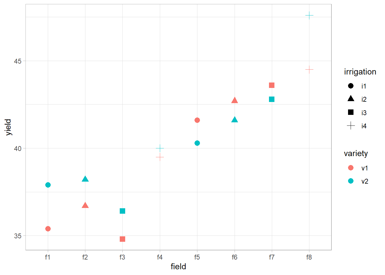

sp_model <-
    lmerTest::lmer(yield ~ irrigation * variety 
                   + (1 |field), irrigation)
summary(sp_model)
#> Linear mixed model fit by REML. t-tests use Satterthwaite's method [
#> lmerModLmerTest]
#> Formula: yield ~ irrigation * variety + (1 | field)
#>    Data: irrigation
#> 
#> REML criterion at convergence: 45.4
#> 
#> Scaled residuals: 
#>     Min      1Q  Median      3Q     Max 
#> -0.7448 -0.5509  0.0000  0.5509  0.7448 
#> 
#> Random effects:
#>  Groups   Name        Variance Std.Dev.
#>  field    (Intercept) 16.200   4.025   
#>  Residual              2.107   1.452   
#> Number of obs: 16, groups:  field, 8
#> 
#> Fixed effects:
#>                        Estimate Std. Error     df t value Pr(>|t|)    
#> (Intercept)              38.500      3.026  4.487  12.725 0.000109 ***
#> irrigationi2              1.200      4.279  4.487   0.280 0.791591    
#> irrigationi3              0.700      4.279  4.487   0.164 0.877156    
#> irrigationi4              3.500      4.279  4.487   0.818 0.454584    
#> varietyv2                 0.600      1.452  4.000   0.413 0.700582    
#> irrigationi2:varietyv2   -0.400      2.053  4.000  -0.195 0.855020    
#> irrigationi3:varietyv2   -0.200      2.053  4.000  -0.097 0.927082    
#> irrigationi4:varietyv2    1.200      2.053  4.000   0.584 0.590265    
#> ---
#> Signif. codes:  0 '***' 0.001 '**' 0.01 '*' 0.05 '.' 0.1 ' ' 1
#> 
#> Correlation of Fixed Effects:
#>             (Intr) irrgt2 irrgt3 irrgt4 vrtyv2 irr2:2 irr3:2
#> irrigation2 -0.707                                          
#> irrigation3 -0.707  0.500                                   
#> irrigation4 -0.707  0.500  0.500                            
#> varietyv2   -0.240  0.170  0.170  0.170                     
#> irrgtn2:vr2  0.170 -0.240 -0.120 -0.120 -0.707              
#> irrgtn3:vr2  0.170 -0.120 -0.240 -0.120 -0.707  0.500       
#> irrgtn4:vr2  0.170 -0.120 -0.120 -0.240 -0.707  0.500  0.500

anova(sp_model, ddf = c("Kenward-Roger"))
#> Type III Analysis of Variance Table with Kenward-Roger's method
#>                    Sum Sq Mean Sq NumDF DenDF F value Pr(>F)
#> irrigation         2.4545 0.81818     3     4  0.3882 0.7685
#> variety            2.2500 2.25000     1     4  1.0676 0.3599
#> irrigation:variety 1.5500 0.51667     3     4  0.2452 0.8612

Since p-value of the interaction term is insignificant, we consider fitting without it.

library(lme4)
sp_model_additive <- lmer(yield ~ irrigation + variety 
                          + (1 | field), irrigation)
anova(sp_model_additive,sp_model,ddf = "Kenward-Roger")
#> Data: irrigation
#> Models:
#> sp_model_additive: yield ~ irrigation + variety + (1 | field)
#> sp_model: yield ~ irrigation * variety + (1 | field)
#>                   npar    AIC    BIC  logLik deviance  Chisq Df Pr(>Chisq)
#> sp_model_additive    7 83.959 89.368 -34.980   69.959                     
#> sp_model            10 88.609 96.335 -34.305   68.609 1.3503  3     0.7172

Since \(p\)-value of \(\chi^2\) test is insignificant, we can’t reject the additive model is already sufficient. Looking at AIC and BIC, we can also see that we would prefer the additive model

Random Effect Examination

exactRLRT test

• \(H_0\): Var(random effect) (i.e., \(\sigma^2\))= 0
• \(H_a\): Var(random effect) (i.e., \(\sigma^2\)) > 0

sp_model <- lme4::lmer(yield ~ irrigation * variety 
                       + (1 | field), irrigation)
library(RLRsim)
exactRLRT(sp_model)
#> 
#>  simulated finite sample distribution of RLRT.
#>  
#>  (p-value based on 10000 simulated values)
#> 
#> data:  
#> RLRT = 6.1118, p-value = 0.0087

Since the p-value is significant, we reject \(H_0\)

8.6 Repeated Measures in Mixed Models

\[ Y_{ijk} = \mu + \alpha_i + \beta_j + (\alpha \beta)_{ij} + \delta_{i(k)}+ \epsilon_{ijk} \]

where

• \(i\)-th group (fixed)
• \(j\)-th (repeated measure) time effect (fixed)
• \(k\)-th subject
• \(\delta_{i(k)} \sim N(0,\sigma^2_\delta)\) (k-th subject in the \(i\)-th group) and \(\epsilon_{ijk} \sim N(0,\sigma^2)\) (independent error) are random effects (\(i = 1,..,n_A, j = 1,..,n_B, k = 1,...,n_i\))

hence, the variance-covariance matrix of the repeated observations on the k-th subject of the i-th group, \(\mathbf{Y}_{ik} = (Y_{i1k},..,Y_{in_Bk})'\), will be

\[ \begin{aligned} \mathbf{\Sigma}_{subject} &= \left( \begin{array} {cccc} \sigma^2_\delta + \sigma^2 & \sigma^2_\delta & ... & \sigma^2_\delta \\ \sigma^2_\delta & \sigma^2_\delta +\sigma^2 & ... & \sigma^2_\delta \\ . & . & . & . \\ \sigma^2_\delta & \sigma^2_\delta & ... & \sigma^2_\delta + \sigma^2 \\ \end{array} \right) \\ &= (\sigma^2_\delta + \sigma^2) \left( \begin{array} {cccc} 1 & \rho & ... & \rho \\ \rho & 1 & ... & \rho \\ . & . & . & . \\ \rho & \rho & ... & 1 \\ \end{array} \right) & \text{product of a scalar and a correlation matrix} \end{aligned} \]

where \(\rho = \frac{\sigma^2_\delta}{\sigma^2_\delta + \sigma^2}\), which is the compound symmetry structure that we discussed in Random-Intercepts Model

But if you only have repeated measurements on the subject over time, AR(1) structure might be more appropriate

Mixed model for a repeated measure

\[ Y_{ijk} = \mu + \alpha_i + \beta_j + (\alpha \beta)_{ij} + \epsilon_{ijk} \]

where

• \(\epsilon_{ijk}\) combines random error of both the whole and subplots.

In general,

\[ \mathbf{Y = X \beta + \epsilon} \]

where

• \(\epsilon \sim N(0, \sigma^2 \mathbf{\Sigma})\) where \(\mathbf{\Sigma}\) is block diagonal if the random error covariance is the same for each subject

The variance covariance matrix with AR(1) structure is

\[ \mathbf{\Sigma}_{subject} = \sigma^2 \left( \begin{array} {ccccc} 1 & \rho & \rho^2 & ... & \rho^{n_B-1} \\ \rho & 1 & \rho & ... & \rho^{n_B-2} \\ . & . & . & . & . \\ \rho^{n_B-1} & \rho^{n_B-2} & \rho^{n_B-3} & ... & 1 \\ \end{array} \right) \]

Hence, the mixed model for a repeated measure can be written as

\[ Y_{ijk} = \mu + \alpha_i + \beta_j + (\alpha \beta)_{ij} + \epsilon_{ijk} \]

where

• \(\epsilon_{ijk}\) = random error of whole and subplots

Generally,

\[ \mathbf{Y = X \beta + \epsilon} \]

where \(\epsilon \sim N(0, \mathbf{\sigma^2 \Sigma})\) and \(\Sigma\) = block diagonal if the random error covariance is the same for each subject.

8.7 Unbalanced or Unequally Spaced Data

Consider the model

\[ Y_{ikt} = \beta_0 + \beta_{0i} + \beta_{1}t + \beta_{1i}t + \beta_{2} t^2 + \beta_{2i} t^2 + \epsilon_{ikt} \]

where

• \(i = 1,2\) (groups)
• \(k = 1,…, n_i\) ( individuals)
• \(t = (t_1,t_2,t_3,t_4)\) (times)
• \(\beta_{2i}\) = common quadratic term
• \(\beta_{1i}\) = common linear time trends
• \(\beta_{0i}\) = common intercepts

Then, we assume the variance-covariance matrix of the repeated measurements collected on a particular subject over time has the form

\[ \mathbf{\Sigma}_{ik} = \sigma^2 \left( \begin{array} {cccc} 1 & \rho^{t_2-t_1} & \rho^{t_3-t_1} & \rho^{t_4-t_1} \\ \rho^{t_2-t_1} & 1 & \rho^{t_3-t_2} & \rho^{t_4-t_2} \\ \rho^{t_3-t_1} & \rho^{t_3-t_2} & 1 & \rho^{t_4-t_3} \\ \rho^{t_4-t_1} & \rho^{t_4-t_2} & \rho^{t_4-t_3} & 1 \end{array} \right) \]

which is called “power” covariance model

We can consider \(\beta_{2i} , \beta_{1i}, \beta_{0i}\) accordingly to see whether these terms are needed in the final model

8.8 Application

R Packages for mixed models

• nlme

  • has nested structure

  • flexible for complex design

  • not user-friendly

• lme4

  • computationally efficient

  • user-friendly

  • can handle non-normal response

  • for more detailed application, check Fitting Linear Mixed-Effects Models Using lme4

• Others

  • Bayesian setting: MCMCglmm, brms

  • For genetics: ASReml

8.8.1 Example 1 (Pulps)

Model:

\[ y_{ij} = \mu + \alpha_i + \epsilon_{ij} \]

where

• \(i = 1,..,a\) groups for random effect \(\alpha_i\)
• \(j = 1,...,n\) individuals in each group
• \(\alpha_i \sim N(0, \sigma^2_\alpha)\) is random effects
• \(\epsilon_{ij} \sim N(0, \sigma^2_\epsilon)\) is random effects
• Imply compound symmetry model where the intraclass correlation coefficient is: \(\rho = \frac{\sigma^2_\alpha}{\sigma^2_\alpha + \sigma^2_\epsilon}\)
• If factor \(a\) does not explain much variation, low correlation within the levels: \(\sigma^2_\alpha \to 0\) then \(\rho \to 0\)
• If factor \(a\) explain much variation, high correlation within the levels \(\sigma^2_\alpha \to \infty\) hence, \(\rho \to 1\)

data(pulp, package = "faraway")
plot(
    y    = pulp$bright,
    x    = pulp$operator,
    xlab = "Operator",
    ylab = "Brightness"
)

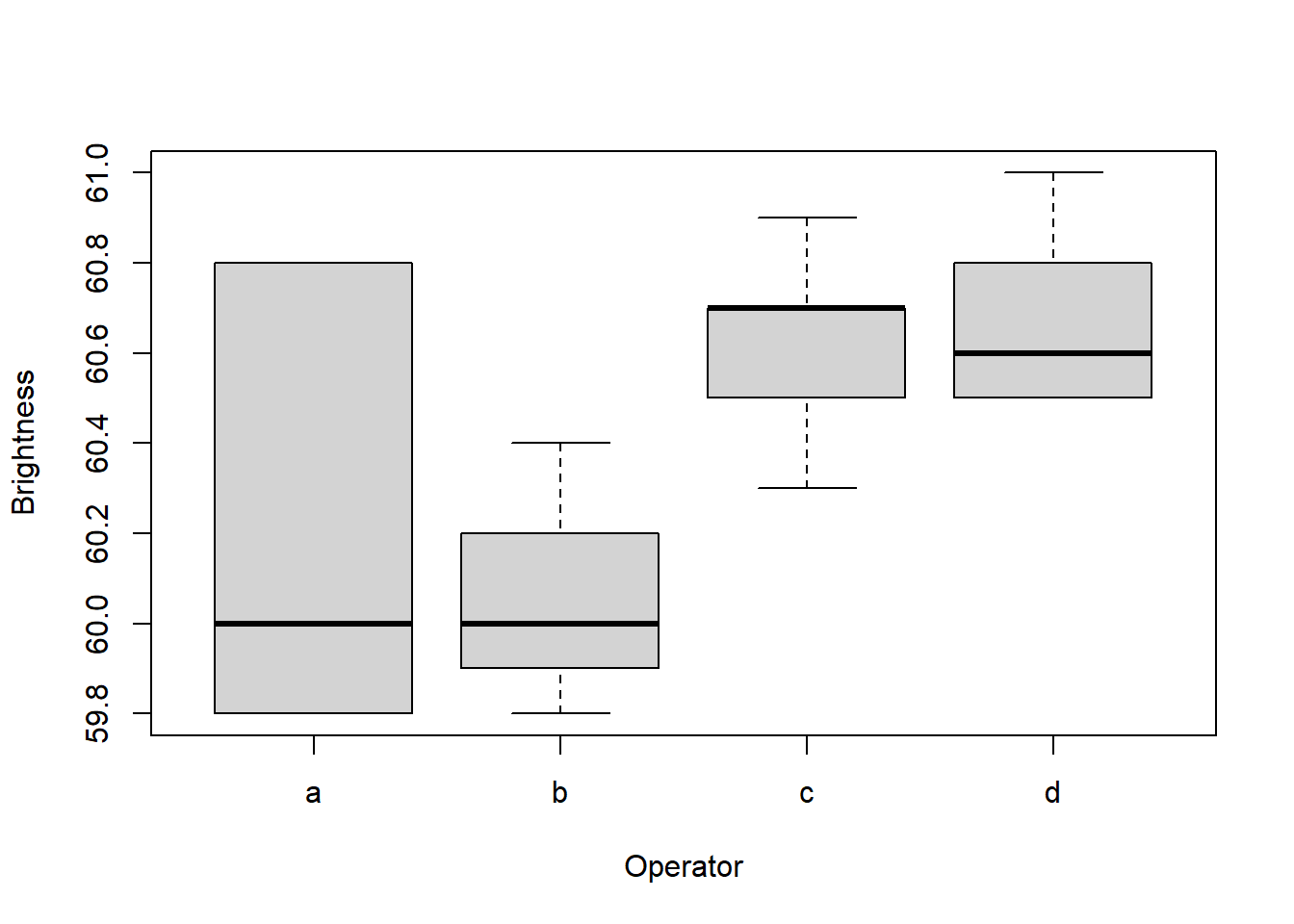
pulp %>% dplyr::group_by(operator) %>% 
    dplyr::summarise(average = mean(bright))
#> # A tibble: 4 × 2
#>   operator average
#>   <fct>      <dbl>
#> 1 a           60.2
#> 2 b           60.1
#> 3 c           60.6
#> 4 d           60.7

lmer application

library(lme4)
mixed_model <-
    lmer(
        # pipe (i..e, | ) denotes random-effect terms
        formula = bright ~ 1 + (1 |operator), 
         data = pulp)
summary(mixed_model)
#> Linear mixed model fit by REML ['lmerMod']
#> Formula: bright ~ 1 + (1 | operator)
#>    Data: pulp
#> 
#> REML criterion at convergence: 18.6
#> 
#> Scaled residuals: 
#>     Min      1Q  Median      3Q     Max 
#> -1.4666 -0.7595 -0.1244  0.6281  1.6012 
#> 
#> Random effects:
#>  Groups   Name        Variance Std.Dev.
#>  operator (Intercept) 0.06808  0.2609  
#>  Residual             0.10625  0.3260  
#> Number of obs: 20, groups:  operator, 4
#> 
#> Fixed effects:
#>             Estimate Std. Error t value
#> (Intercept)  60.4000     0.1494   404.2
coef(mixed_model)
#> $operator
#>   (Intercept)
#> a    60.27806
#> b    60.14088
#> c    60.56767
#> d    60.61340
#> 
#> attr(,"class")
#> [1] "coef.mer"
fixef(mixed_model)   # fixed effects
#> (Intercept) 
#>        60.4
confint(mixed_model) # confidence interval
#>                 2.5 %     97.5 %
#> .sig01       0.000000  0.6178987
#> .sigma       0.238912  0.4821845
#> (Intercept) 60.071299 60.7287012
ranef(mixed_model)   # random effects
#> $operator
#>   (Intercept)
#> a  -0.1219403
#> b  -0.2591231
#> c   0.1676679
#> d   0.2133955
#> 
#> with conditional variances for "operator"
VarCorr(mixed_model) # random effects standard deviation
#>  Groups   Name        Std.Dev.
#>  operator (Intercept) 0.26093 
#>  Residual             0.32596
re_dat = as.data.frame(VarCorr(mixed_model))

# rho based on the above formula
rho = re_dat[1, 'vcov'] / (re_dat[1, 'vcov'] + re_dat[2, 'vcov'])
rho
#> [1] 0.3905354

To Satterthwaite approximation for the denominator df, we use lmerTest

library(lmerTest)
summary(lmerTest::lmer(bright ~ 1 + (1 | operator), pulp))$coefficients
#>             Estimate Std. Error df  t value     Pr(>|t|)
#> (Intercept)     60.4  0.1494434  3 404.1664 3.340265e-08
confint(mixed_model)[3, ]
#>   2.5 %  97.5 % 
#> 60.0713 60.7287

In this example, we can see that the confidence interval computed by confint in lmer package is very close is confint in lmerTest model.

MCMglmm application

under the Bayesian framework

library(MCMCglmm)
mixed_model_bayes <-
    MCMCglmm(
        bright ~ 1,
        random =  ~ operator,
        data = pulp,
        verbose = FALSE
    )
summary(mixed_model_bayes)$solutions
#>             post.mean l-95% CI u-95% CI eff.samp pMCMC
#> (Intercept)  60.40449  60.2055 60.66595     1000 0.001

this method offers the confidence interval slightly more positive than lmer and lmerTest

8.8.1.1 Prediction

# random effects prediction (BLUPs)
ranef(mixed_model)$operator
#>   (Intercept)
#> a  -0.1219403
#> b  -0.2591231
#> c   0.1676679
#> d   0.2133955

# prediction for each categories
fixef(mixed_model) + ranef(mixed_model)$operator 
#>   (Intercept)
#> a    60.27806
#> b    60.14088
#> c    60.56767
#> d    60.61340

# equivalent to the above method
predict(mixed_model, newdata = data.frame(operator = c('a', 'b', 'c', 'd'))) 
#>        1        2        3        4 
#> 60.27806 60.14088 60.56767 60.61340

use bootMer() to get bootstrap-based confidence intervals for predictions.

Another example using GLMM in the context of blocking

Penicillin data

data(penicillin, package = "faraway")
summary(penicillin)
#>  treat    blend       yield   
#>  A:5   Blend1:4   Min.   :77  
#>  B:5   Blend2:4   1st Qu.:81  
#>  C:5   Blend3:4   Median :87  
#>  D:5   Blend4:4   Mean   :86  
#>        Blend5:4   3rd Qu.:89  
#>                   Max.   :97
library(ggplot2)
ggplot(penicillin, aes(
    y     = yield,
    x     = treat,
    shape = blend,
    color = blend
)) + 
    # treatment = fixed effect
    # blend = random effects
    geom_point(size = 3) +
    xlab("Treatment")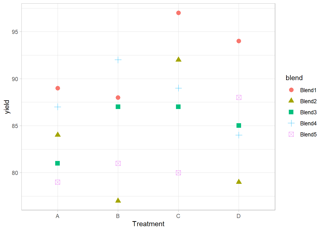

library(lmerTest) # for p-values
mixed_model <- lmerTest::lmer(yield ~ treat + (1 | blend),
                              data = penicillin)
summary(mixed_model)
#> Linear mixed model fit by REML. t-tests use Satterthwaite's method [
#> lmerModLmerTest]
#> Formula: yield ~ treat + (1 | blend)
#>    Data: penicillin
#> 
#> REML criterion at convergence: 103.8
#> 
#> Scaled residuals: 
#>     Min      1Q  Median      3Q     Max 
#> -1.4152 -0.5017 -0.1644  0.6830  1.2836 
#> 
#> Random effects:
#>  Groups   Name        Variance Std.Dev.
#>  blend    (Intercept) 11.79    3.434   
#>  Residual             18.83    4.340   
#> Number of obs: 20, groups:  blend, 5
#> 
#> Fixed effects:
#>             Estimate Std. Error     df t value Pr(>|t|)    
#> (Intercept)   84.000      2.475 11.075  33.941 1.51e-12 ***
#> treatB         1.000      2.745 12.000   0.364   0.7219    
#> treatC         5.000      2.745 12.000   1.822   0.0935 .  
#> treatD         2.000      2.745 12.000   0.729   0.4802    
#> ---
#> Signif. codes:  0 '***' 0.001 '**' 0.01 '*' 0.05 '.' 0.1 ' ' 1
#> 
#> Correlation of Fixed Effects:
#>        (Intr) treatB treatC
#> treatB -0.555              
#> treatC -0.555  0.500       
#> treatD -0.555  0.500  0.500

#The BLUPs for the each blend
ranef(mixed_model)$blend
#>        (Intercept)
#> Blend1   4.2878788
#> Blend2  -2.1439394
#> Blend3  -0.7146465
#> Blend4   1.4292929
#> Blend5  -2.8585859

Examine treatment effect

anova(mixed_model) # p-value based on lmerTest
#> Type III Analysis of Variance Table with Satterthwaite's method
#>       Sum Sq Mean Sq NumDF DenDF F value Pr(>F)
#> treat     70  23.333     3    12  1.2389 0.3387

Since the p-value is greater than 0.05, we can’t reject the null hypothesis that there is no treatment effect.

library(pbkrtest)
# REML is not appropriate for testing fixed effects, it should be ML
full_model <-
    lmer(yield ~ treat + (1 | blend), 
         penicillin, 
         REML = FALSE) 
null_model <- lmer(yield ~ 1 + (1 | blend), 
                   penicillin, 
                   REML = FALSE)

# use  Kenward-Roger approximation for df
KRmodcomp(full_model, null_model) 
#> large : yield ~ treat + (1 | blend)
#> small : yield ~ 1 + (1 | blend)
#>          stat     ndf     ddf F.scaling p.value
#> Ftest  1.2389  3.0000 12.0000         1  0.3387

Since the p-value is greater than 0.05, and consistent with our previous observation, we conclude that we can’t reject the null hypothesis that there is no treatment effect.

8.8.2 Example 2 (Rats)

rats <- read.csv(
    "images/rats.dat",
    header = F,
    sep = ' ',
    col.names = c('Treatment', 'rat', 'age', 'y')
)

# log transformed age
rats$t <- log(1 + (rats$age - 45) / 10) 

We are interested in whether treatment effect induces changes over time.

rat_model <-
    # treatment = fixed effect, rat = random effects
    lmerTest::lmer(y ~ t:Treatment + (1 | rat), 
                   data = rats) 
summary(rat_model)
#> Linear mixed model fit by REML. t-tests use Satterthwaite's method [
#> lmerModLmerTest]
#> Formula: y ~ t:Treatment + (1 | rat)
#>    Data: rats
#> 
#> REML criterion at convergence: 932.4
#> 
#> Scaled residuals: 
#>      Min       1Q   Median       3Q      Max 
#> -2.25574 -0.65898 -0.01163  0.58356  2.88309 
#> 
#> Random effects:
#>  Groups   Name        Variance Std.Dev.
#>  rat      (Intercept) 3.565    1.888   
#>  Residual             1.445    1.202   
#> Number of obs: 252, groups:  rat, 50
#> 
#> Fixed effects:
#>                Estimate Std. Error       df t value Pr(>|t|)    
#> (Intercept)     68.6074     0.3312  89.0275  207.13   <2e-16 ***
#> t:Treatmentcon   7.3138     0.2808 247.2762   26.05   <2e-16 ***
#> t:Treatmenthig   6.8711     0.2276 247.7097   30.19   <2e-16 ***
#> t:Treatmentlow   7.5069     0.2252 247.5196   33.34   <2e-16 ***
#> ---
#> Signif. codes:  0 '***' 0.001 '**' 0.01 '*' 0.05 '.' 0.1 ' ' 1
#> 
#> Correlation of Fixed Effects:
#>             (Intr) t:Trtmntc t:Trtmnth
#> t:Tretmntcn -0.327                    
#> t:Tretmnthg -0.340  0.111             
#> t:Tretmntlw -0.351  0.115     0.119
anova(rat_model)
#> Type III Analysis of Variance Table with Satterthwaite's method
#>             Sum Sq Mean Sq NumDF  DenDF F value    Pr(>F)    
#> t:Treatment 3181.9  1060.6     3 223.21  734.11 < 2.2e-16 ***
#> ---
#> Signif. codes:  0 '***' 0.001 '**' 0.01 '*' 0.05 '.' 0.1 ' ' 1

Since the p-value is significant, we can be confident concluding that there is a treatment effect

8.8.3 Example 3 (Agridat)

library(agridat)
library(latticeExtra)
dat <- harris.wateruse
# Compare to Schabenberger & Pierce, fig 7.23
useOuterStrips(
    xyplot(
        water ~ day | species * age,
        dat,
        as.table = TRUE,
        group = tree,
        type = c('p', 'smooth'),
        main = "harris.wateruse 2 species, 2 ages (10 trees each)"
    )
)

Remove outliers

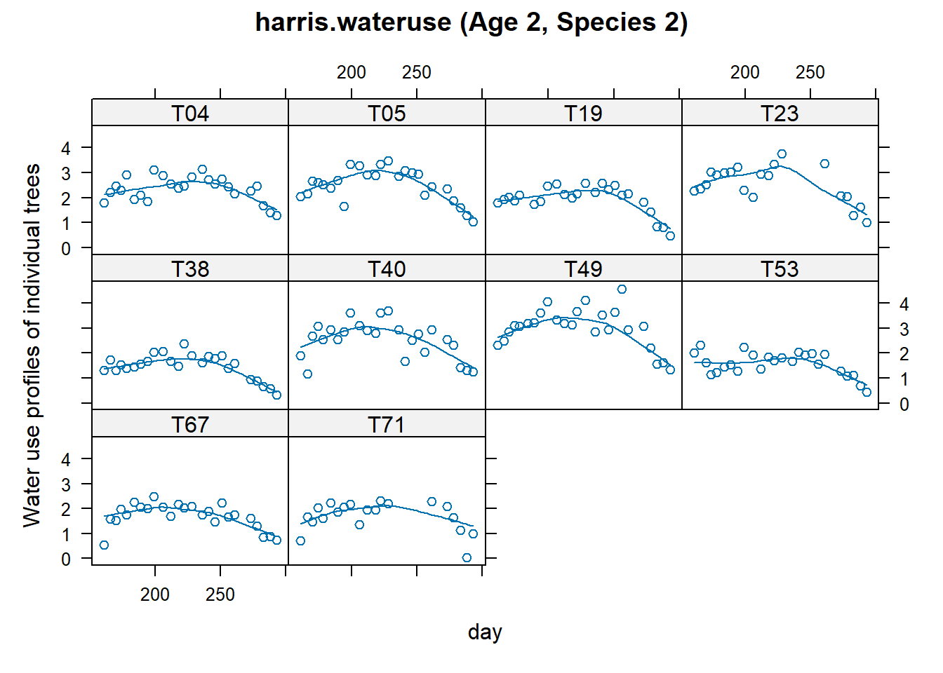
dat <- subset(dat, day!=268)

Plot between age and species

xyplot(
    water ~ day | tree,
    dat,
    subset   = age == "A2" & species == "S2",
    as.table = TRUE,
    type     = c('p', 'smooth'),
    ylab     = "Water use profiles of individual trees",
    main     = "harris.wateruse (Age 2, Species 2)"
)

# Rescale day for nicer output, 
# and convergence issues, add quadratic term
dat <- transform(dat, ti = day / 100)
dat <- transform(dat, ti2 = ti * ti)
# Start with a subgroup: age 2, species 2
d22 <- droplevels(subset(dat, age == "A2" & species == "S2"))

lme function from nlme package

library(nlme)

## We use pdDiag() to get uncorrelated random effects
m1n <- lme(
    water ~ 1 + ti + ti2,
    #intercept, time and time-squared = fixed effects
    data = d22,
    na.action = na.omit,
    random = list(tree = pdDiag(~ 1 + ti + ti2)) 
    # random intercept, time 
    # and time squared per tree = random effects
)
ranef(m1n)
#>     (Intercept)            ti           ti2
#> T04   0.1985796  1.609864e-09  4.990101e-10
#> T05   0.3492827  2.487690e-10 -4.845287e-11
#> T19  -0.1978989 -7.681202e-10 -1.961453e-10
#> T23   0.4519003 -3.270426e-10 -2.413583e-10
#> T38  -0.6457494 -1.608770e-09 -3.298010e-10
#> T40   0.3739432  3.264705e-10 -2.543109e-11
#> T49   0.8620648  9.021831e-10 -5.402247e-12
#> T53  -0.5655049 -8.279040e-10 -4.579291e-11
#> T67  -0.4394623 -3.485113e-10  2.147434e-11
#> T71  -0.3871552  7.930610e-10  3.718993e-10

fixef(m1n)
#> (Intercept)          ti         ti2 
#>  -10.798799   12.346704   -2.838503
summary(m1n)
#> Linear mixed-effects model fit by REML
#>   Data: d22 
#>        AIC     BIC    logLik
#>   276.5142 300.761 -131.2571
#> 
#> Random effects:
#>  Formula: ~1 + ti + ti2 | tree
#>  Structure: Diagonal
#>         (Intercept)           ti          ti2  Residual
#> StdDev:   0.5187869 1.438333e-05 3.864019e-06 0.3836614
#> 
#> Fixed effects:  water ~ 1 + ti + ti2 
#>                  Value Std.Error  DF   t-value p-value
#> (Intercept) -10.798799 0.8814666 227 -12.25094       0
#> ti           12.346704 0.7827112 227  15.77428       0
#> ti2          -2.838503 0.1720614 227 -16.49704       0
#>  Correlation: 
#>     (Intr) ti    
#> ti  -0.979       
#> ti2  0.970 -0.997
#> 
#> Standardized Within-Group Residuals:
#>         Min          Q1         Med          Q3         Max 
#> -3.07588246 -0.58531056  0.01210209  0.65402695  3.88777402 
#> 
#> Number of Observations: 239
#> Number of Groups: 10

lmer function from lme4 package

m1lmer <-
    lmer(water ~ 1 + ti + ti2 + (ti + ti2 ||
                                     tree),
         data = d22,
         na.action = na.omit)
ranef(m1lmer)
#> $tree
#>     (Intercept) ti ti2
#> T04   0.1985796  0   0
#> T05   0.3492827  0   0
#> T19  -0.1978989  0   0
#> T23   0.4519003  0   0
#> T38  -0.6457494  0   0
#> T40   0.3739432  0   0
#> T49   0.8620648  0   0
#> T53  -0.5655049  0   0
#> T67  -0.4394623  0   0
#> T71  -0.3871552  0   0
#> 
#> with conditional variances for "tree"

Notes:

• || double pipes= uncorrelated random effects

• To remove the intercept term:

  • (0+ti|tree)

  • (ti-1|tree)

fixef(m1lmer)
#> (Intercept)          ti         ti2 
#>  -10.798799   12.346704   -2.838503
m1l <-
    lmer(water ~ 1 + ti + ti2 
         + (1 | tree) + (0 + ti | tree) 
         + (0 + ti2 | tree), data = d22)
ranef(m1l)
#> $tree
#>     (Intercept) ti ti2
#> T04   0.1985796  0   0
#> T05   0.3492827  0   0
#> T19  -0.1978989  0   0
#> T23   0.4519003  0   0
#> T38  -0.6457494  0   0
#> T40   0.3739432  0   0
#> T49   0.8620648  0   0
#> T53  -0.5655049  0   0
#> T67  -0.4394623  0   0
#> T71  -0.3871552  0   0
#> 
#> with conditional variances for "tree"
fixef(m1l)
#> (Intercept)          ti         ti2 
#>  -10.798799   12.346704   -2.838503

To include structured covariance terms, we can use the following way

m2n <- lme(
    water ~ 1 + ti + ti2,
    data = d22,
    random = ~ 1 | tree,
    cor = corExp(form =  ~ day | tree),
    na.action = na.omit
)
ranef(m2n)
#>     (Intercept)
#> T04   0.1929971
#> T05   0.3424631
#> T19  -0.1988495
#> T23   0.4538660
#> T38  -0.6413664
#> T40   0.3769378
#> T49   0.8410043
#> T53  -0.5528236
#> T67  -0.4452930
#> T71  -0.3689358
fixef(m2n)
#> (Intercept)          ti         ti2 
#>  -11.223310   12.712094   -2.913682
summary(m2n)
#> Linear mixed-effects model fit by REML
#>   Data: d22 
#>        AIC      BIC   logLik
#>   263.3081 284.0911 -125.654
#> 
#> Random effects:
#>  Formula: ~1 | tree
#>         (Intercept)  Residual
#> StdDev:   0.5154042 0.3925777
#> 
#> Correlation Structure: Exponential spatial correlation
#>  Formula: ~day | tree 
#>  Parameter estimate(s):
#>    range 
#> 3.794624 
#> Fixed effects:  water ~ 1 + ti + ti2 
#>                  Value Std.Error  DF   t-value p-value
#> (Intercept) -11.223310 1.0988725 227 -10.21348       0
#> ti           12.712094 0.9794235 227  12.97916       0
#> ti2          -2.913682 0.2148551 227 -13.56115       0
#>  Correlation: 
#>     (Intr) ti    
#> ti  -0.985       
#> ti2  0.976 -0.997
#> 
#> Standardized Within-Group Residuals:
#>         Min          Q1         Med          Q3         Max 
#> -3.04861039 -0.55703950  0.00278101  0.62558762  3.80676991 
#> 
#> Number of Observations: 239
#> Number of Groups: 10