7.4 Poisson Regression
From the Poisson distribution
\[ \begin{aligned} f(Y_i) &= \frac{\mu_i^{Y_i}exp(-\mu_i)}{Y_i!}, Y_i = 0,1,.. \\ E(Y_i) &= \mu_i \\ var(Y_i) &= \mu_i \end{aligned} \]
which is a natural distribution for counts. We can see that the variance is a function of the mean. If we let \(\mu_i = f(\mathbf{x_i; \theta})\), it would be similar to Logistic Regression since we can choose \(f()\) as \(\mu_i = \mathbf{x_i'\theta}, \mu_i = \exp(\mathbf{x_i'\theta}), \mu_i = \log(\mathbf{x_i'\theta})\)
7.4.1 Application
Count Data and Poisson regression
data(bioChemists, package = "pscl")
bioChemists <- bioChemists %>%
    rename(
        Num_Article = art, #articles in last 3 years of PhD
        Sex = fem, #coded 1 if female
        Married = mar, #coded 1 if married
        Num_Kid5 = kid5, #number of childeren under age 6
        PhD_Quality = phd, #prestige of PhD program
        Num_MentArticle = ment #articles by mentor in last 3 years
    )
hist(bioChemists$Num_Article, breaks = 25, main = 'Number of Articles')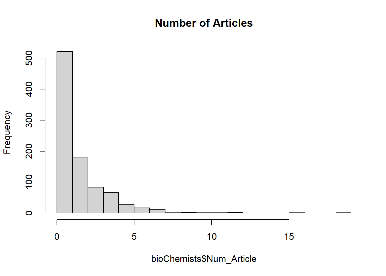
Poisson_Mod <- glm(Num_Article ~ ., family=poisson, bioChemists)
summary(Poisson_Mod)
#>
#> Call:
#> glm(formula = Num_Article ~ ., family = poisson, data = bioChemists)
#>
#> Deviance Residuals:
#>     Min       1Q   Median       3Q      Max
#> -3.5672  -1.5398  -0.3660   0.5722   5.4467
#>
#> Coefficients:
#>                  Estimate Std. Error z value Pr(>|z|)
#> (Intercept)      0.304617   0.102981   2.958   0.0031 **
#> SexWomen        -0.224594   0.054613  -4.112 3.92e-05 ***
#> MarriedMarried   0.155243   0.061374   2.529   0.0114 *
#> Num_Kid5        -0.184883   0.040127  -4.607 4.08e-06 ***
#> PhD_Quality      0.012823   0.026397   0.486   0.6271
#> Num_MentArticle  0.025543   0.002006  12.733  < 2e-16 ***
#> ---
#> Signif. codes:  0 '***' 0.001 '**' 0.01 '*' 0.05 '.' 0.1 ' ' 1
#>
#> (Dispersion parameter for poisson family taken to be 1)
#>
#>     Null deviance: 1817.4  on 914  degrees of freedom
#> Residual deviance: 1634.4  on 909  degrees of freedom
#> AIC: 3314.1
#>
#> Number of Fisher Scoring iterations: 5
Residual of 1634 with 909 df isn’t great.
We see Pearson \(\chi^2\)
Predicted_Means <- predict(Poisson_Mod,type = "response")
X2 <- sum((bioChemists$Num_Article - Predicted_Means)^2/Predicted_Means)
X2
#> [1] 1662.547
pchisq(X2,Poisson_Mod$df.residual, lower.tail = FALSE)
#> [1] 7.849882e-47
With interaction terms, there are some improvements
Poisson_Mod_All2way <- glm(Num_Article ~ .^2, family=poisson, bioChemists)
Poisson_Mod_All3way <- glm(Num_Article ~ .^3, family=poisson, bioChemists)
Consider the \(\hat{\phi} = \frac{\text{deviance}}{df}\)
This is evidence for over-dispersion. Likely cause is missing variables. And remedies could either be to include more variables or consider random effects.
A quick fix is to force the Poisson Regression to include this value of \(\phi\), and this model is called “Quasi-Poisson”.
phi_hat = Poisson_Mod$deviance/Poisson_Mod$df.residual
summary(Poisson_Mod,dispersion = phi_hat)
#>
#> Call:
#> glm(formula = Num_Article ~ ., family = poisson, data = bioChemists)
#>
#> Deviance Residuals:
#>     Min       1Q   Median       3Q      Max
#> -3.5672  -1.5398  -0.3660   0.5722   5.4467
#>
#> Coefficients:
#>                 Estimate Std. Error z value Pr(>|z|)
#> (Intercept)      0.30462    0.13809   2.206  0.02739 *
#> SexWomen        -0.22459    0.07323  -3.067  0.00216 **
#> MarriedMarried   0.15524    0.08230   1.886  0.05924 .
#> Num_Kid5        -0.18488    0.05381  -3.436  0.00059 ***
#> PhD_Quality      0.01282    0.03540   0.362  0.71715
#> Num_MentArticle  0.02554    0.00269   9.496  < 2e-16 ***
#> ---
#> Signif. codes:  0 '***' 0.001 '**' 0.01 '*' 0.05 '.' 0.1 ' ' 1
#>
#> (Dispersion parameter for poisson family taken to be 1.797988)
#>
#>     Null deviance: 1817.4  on 914  degrees of freedom
#> Residual deviance: 1634.4  on 909  degrees of freedom
#> AIC: 3314.1
#>
#> Number of Fisher Scoring iterations: 5
Or directly rerun the model as
Quasi-Poisson is not recommended, but Negative Binomial Regression that has an extra parameter to account for over-dispersion is.