7.6 Multinomial
If we have more than two categories or groups that we want to model relative to covariates (e.g., we have observations \(i = 1,…,n\) and groups/ covariates \(j = 1,2,…,J\)), multinomial is our candidate model
Let
- \(p_{ij}\) be the probability that the i-th observation belongs to the j-th group
- \(Y_{ij}\) be the number of observations for individual i in group j; An individual will have observations \(Y_{i1},Y_{i2},…Y_{iJ}\)
- assume the probability of observing this response is given by a multinomial distribution in terms of probabilities \(p_{ij}\), where \(\sum_{j = 1}^J p_{ij} = 1\) . For interpretation, we have a baseline category \(p_{i1} = 1 - \sum_{j = 2}^J p_{ij}\)
The link between the mean response (probability) \(p_{ij}\) and a linear function of the covariates
\[ \eta_{ij} = \mathbf{x'_i \beta_j} = \log \frac{p_{ij}}{p_{i1}}, j = 2,..,J \]
We compare \(p_{ij}\) to the baseline \(p_{i1}\), suggesting
\[ p_{ij} = \frac{\exp(\eta_{ij})}{1 + \sum_{i=2}^J \exp(\eta_{ij})} \]
which is known as multinomial logistic model.
Note:
- Softmax coding for multinomial logistic regression: rather than selecting a baseline class, we treat all \(K\) class symmetrically - equally important (no baseline).
\[ P(Y = k | X = x) = \frac{exp(\beta_{k1} + \dots + \beta_{k_p x_p})}{\sum_{l = 1}^K exp(\beta_{l0} + \dots + \beta_{l_p x_p})} \]
then the log odds ratio between k-th and k’-th classes is
\[ \log (\frac{P(Y=k|X=x)}{P(Y = k' | X=x)}) = (\beta_{k0} - \beta_{k'0}) + \dots + (\beta_{kp} - \beta_{k'p}) x_p \]
library(faraway)
library(dplyr)
data(nes96, package="faraway")
head(nes96,3)
#>   popul TVnews selfLR ClinLR DoleLR     PID age  educ   income    vote
#> 1     0      7 extCon extLib    Con  strRep  36    HS $3Kminus    Dole
#> 2   190      1 sliLib sliLib sliCon weakDem  20  Coll $3Kminus Clinton
#> 3    31      7    Lib    Lib    Con weakDem  24 BAdeg $3Kminus Clinton
We try to understand their political strength
table(nes96$PID)
#>
#>  strDem weakDem  indDem  indind  indRep weakRep  strRep
#>     200     180     108      37      94     150     175
nes96$Political_Strength <- NA
nes96$Political_Strength[nes96$PID %in% c("strDem", "strRep")] <-
    "Strong"
nes96$Political_Strength[nes96$PID %in% c("weakDem", "weakRep")] <-
    "Weak"
nes96$Political_Strength[nes96$PID %in% c("indDem", "indind", "indRep")] <-
    "Neutral"
nes96 %>% group_by(Political_Strength) %>% summarise(Count = n())
#> # A tibble: 3 × 2
#>   Political_Strength Count
#>   <chr>              <int>
#> 1 Neutral              239
#> 2 Strong               375
#> 3 Weak                 330
visualize the political strength variable
library(ggplot2)
Plot_DF <- nes96 %>%
    mutate(Age_Grp = cut_number(age, 4)) %>%
    group_by(Age_Grp, Political_Strength) %>%
    summarise(count = n()) %>%
    group_by(Age_Grp) %>%
    mutate(etotal = sum(count), proportion = count / etotal)

Age_Plot <- ggplot(
    Plot_DF,
    aes(
        x        = Age_Grp,
        y        = proportion,
        group    = Political_Strength,
        linetype = Political_Strength,
        color    = Political_Strength
    )
) +
    geom_line(size = 2)
Age_Plot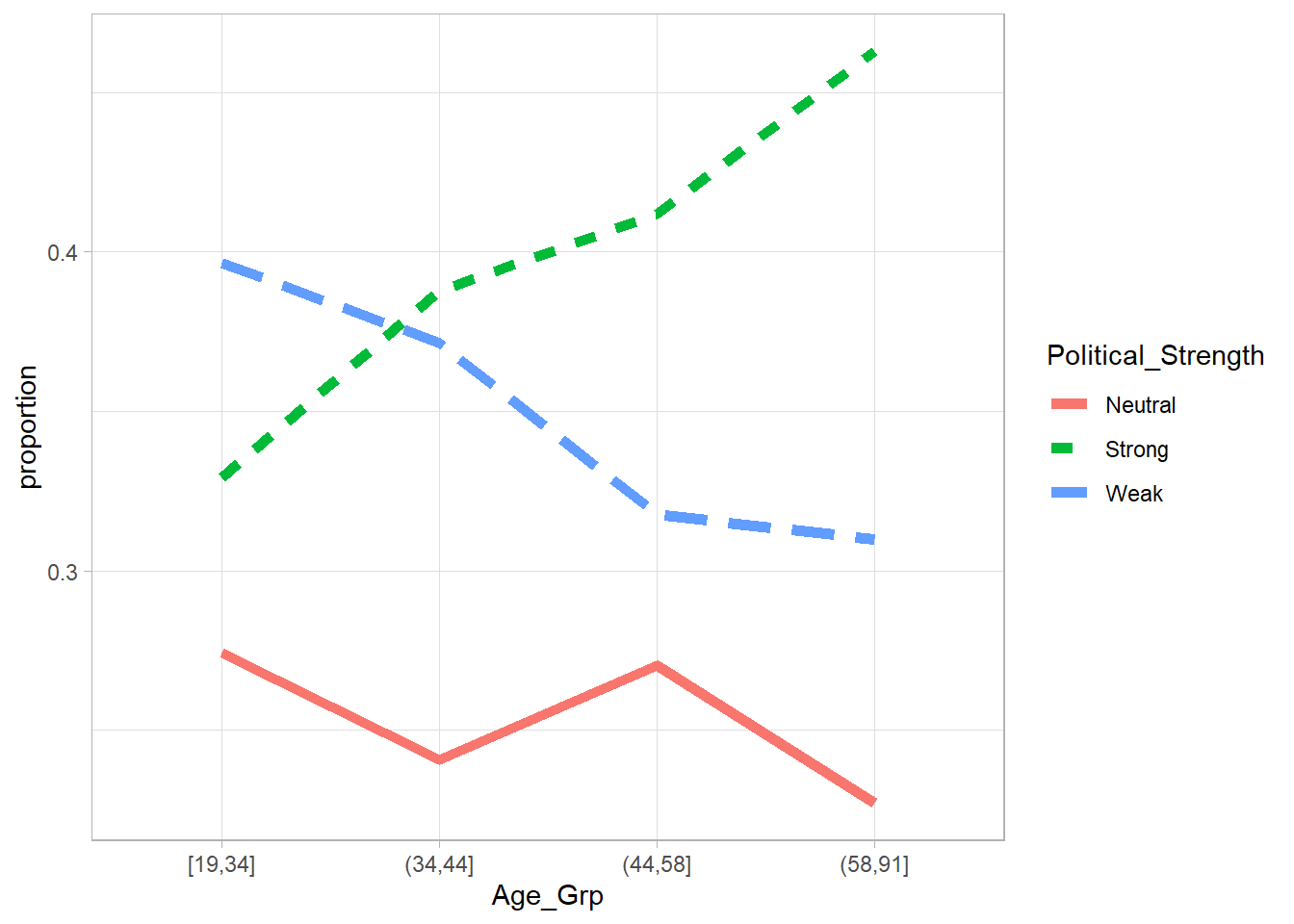
Fit the multinomial logistic model:
model political strength as a function of age and education
library(nnet)
Multinomial_Model <-
    multinom(Political_Strength ~ age + educ, nes96, trace = F)
summary(Multinomial_Model)
#> Call:
#> multinom(formula = Political_Strength ~ age + educ, data = nes96,
#>     trace = F)
#>
#> Coefficients:
#>        (Intercept)          age     educ.L     educ.Q     educ.C      educ^4
#> Strong -0.08788729  0.010700364 -0.1098951 -0.2016197 -0.1757739 -0.02116307
#> Weak    0.51976285 -0.004868771 -0.1431104 -0.2405395 -0.2411795  0.18353634
#>            educ^5     educ^6
#> Strong -0.1664377 -0.1359449
#> Weak   -0.1489030 -0.2173144
#>
#> Std. Errors:
#>        (Intercept)         age    educ.L    educ.Q    educ.C    educ^4
#> Strong   0.3017034 0.005280743 0.4586041 0.4318830 0.3628837 0.2964776
#> Weak     0.3097923 0.005537561 0.4920736 0.4616446 0.3881003 0.3169149
#>           educ^5    educ^6
#> Strong 0.2515012 0.2166774
#> Weak   0.2643747 0.2199186
#>
#> Residual Deviance: 2024.596
#> AIC: 2056.596
Alternatively, stepwise model selection based AIC
Multinomial_Step <- step(Multinomial_Model,trace = 0)
#> trying - age
#> trying - educ
#> trying - age
Multinomial_Step
#> Call:
#> multinom(formula = Political_Strength ~ age, data = nes96, trace = F)
#>
#> Coefficients:
#>        (Intercept)          age
#> Strong -0.01988977  0.009832916
#> Weak    0.59497046 -0.005954348
#>
#> Residual Deviance: 2030.756
#> AIC: 2038.756
compare the best model to the full model based on deviance
pchisq(q = deviance(Multinomial_Step) - deviance(Multinomial_Model),
df = Multinomial_Model$edf-Multinomial_Step$edf,lower=F)
#> [1] 0.9078172
We see no significant difference
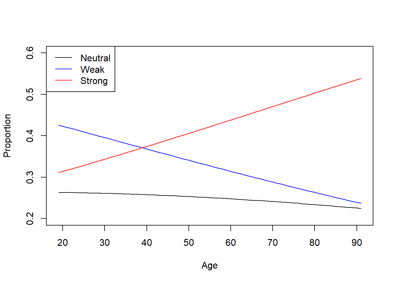
Plot of the fitted model
PlotData <- data.frame(age = seq(from = 19, to = 91))
Preds <-
  PlotData %>% bind_cols(data.frame(predict(
    object = Multinomial_Step,
    PlotData, type = "probs"
  )))

plot(
  x       = Preds$age,
  y       = Preds$Neutral,
  type    = "l",
  ylim    = c(0.2, 0.6),
  col     = "black",
  ylab    = "Proportion",
  xlab    = "Age"
)

lines(x   = Preds$age,
      y   = Preds$Weak,
      col = "blue")
lines(x   = Preds$age,
      y   = Preds$Strong,
      col = "red")

legend(
  'topleft',
  legend  = c('Neutral', 'Weak', 'Strong'),
  col     = c('black', 'blue', 'red'),
  lty     = 1
)
predict(Multinomial_Step,data.frame(age = 34)) # predicted result (categoriy of political strength) of 34 year old
#> [1] Weak
#> Levels: Neutral Strong Weak
predict(Multinomial_Step,data.frame(age = c(34,35)),type="probs") # predicted result of the probabilities of each level of political strength for a 34 and 35
#>     Neutral    Strong      Weak
#> 1 0.2597275 0.3556910 0.3845815
#> 2 0.2594080 0.3587639 0.3818281
If categories are ordered (i.e., ordinal data), we must use another approach (still multinomial, but use cumulative probabilities).
Another example
library(agridat)
dat <- agridat::streibig.competition
# See Schaberger and Pierce, pages 370+
# Consider only the mono-species barley data (no competition from Sinapis)
gammaDat <- subset(dat, sseeds < 1)
gammaDat <-
    transform(gammaDat,
              x = bseeds,
              y = bdwt,
              block = factor(block))
# Inverse yield looks like it will be a good fit for Gamma's inverse link
ggplot(gammaDat, aes(x = x, y = 1 / y)) +
    geom_point(aes(color = block, shape = block)) +
    xlab('Seeding Rate') +
    ylab('Inverse yield') +
    ggtitle('Streibig Competion - Barley only')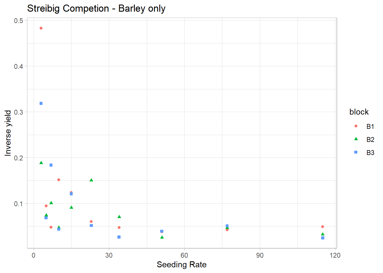
\[ Y \sim Gamma \]
because Gamma is non-negative as opposed to Normal. The canonical Gamma link function is the inverse (or reciprocal) link
\[ \begin{aligned} \eta_{ij} &= \beta_{0j} + \beta_{1j}x_{ij} + \beta_2x_{ij}^2 \\ Y_{ij} &= \eta_{ij}^{-1} \end{aligned} \]
The linear predictor is a quadratic model fit to each of the j-th blocks. A different model (not fitted) could be one with common slopes: glm(y ~ x + I(x^2),…)
# linear predictor is quadratic, with separate intercept and slope per block
m1 <-
glm(y ~ block + block * x + block * I(x ^ 2),
data = gammaDat,
family = Gamma(link = "inverse"))
summary(m1)
#>
#> Call:
#> glm(formula = y ~ block + block * x + block * I(x^2), family = Gamma(link = "inverse"),
#> data = gammaDat)
#>
#> Deviance Residuals:
#> Min 1Q Median 3Q Max
#> -1.21708 -0.44148 0.02479 0.17999 0.80745
#>
#> Coefficients:
#> Estimate Std. Error t value Pr(>|t|)
#> (Intercept) 1.115e-01 2.870e-02 3.886 0.000854 ***
#> blockB2 -1.208e-02 3.880e-02 -0.311 0.758630
#> blockB3 -2.386e-02 3.683e-02 -0.648 0.524029
#> x -2.075e-03 1.099e-03 -1.888 0.072884 .
#> I(x^2) 1.372e-05 9.109e-06 1.506 0.146849
#> blockB2:x 5.198e-04 1.468e-03 0.354 0.726814
#> blockB3:x 7.475e-04 1.393e-03 0.537 0.597103
#> blockB2:I(x^2) -5.076e-06 1.184e-05 -0.429 0.672475
#> blockB3:I(x^2) -6.651e-06 1.123e-05 -0.592 0.560012
#> ---
#> Signif. codes: 0 '***' 0.001 '**' 0.01 '*' 0.05 '.' 0.1 ' ' 1
#>
#> (Dispersion parameter for Gamma family taken to be 0.3232083)
#>
#> Null deviance: 13.1677 on 29 degrees of freedom
#> Residual deviance: 7.8605 on 21 degrees of freedom
#> AIC: 225.32
#>
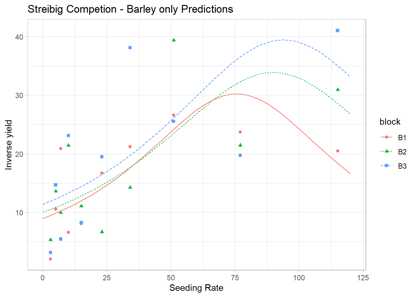
#> Number of Fisher Scoring iterations: 5For predict new value of \(x\)
newdf <-
    expand.grid(x = seq(0, 120, length = 50), block = factor(c('B1', 'B2', 'B3')))

newdf$pred <- predict(m1, new = newdf, type = 'response')

ggplot(gammaDat, aes(x = x, y = y)) +
    geom_point(aes(color = block, shape = block)) +
    xlab('Seeding Rate') + ylab('Inverse yield') +
    ggtitle('Streibig Competion - Barley only Predictions') +
    geom_line(data = newdf, aes(
        x = x,
        y = pred,
        color = block,
        linetype = block
    ))