30.3 Inference
Under just-identified instrument variable model, we have
\[ Y = \beta X + u \]
where \(corr(u, Z) = 0\) (relevant assumption) and \(corr(Z,X) \neq 0\) (exogenous assumption)
The t-ratio approach to construct the 95 CIs is
\[ \hat{\beta} \pm 1.96 \sqrt{\hat{V}_N(\hat{\beta})} \]
But this is wrong, and has been long recognized by those who understand the “weak instruments” problem Dufour (1997)
To test the null hypothesis of \(\beta = \beta_0\) (Lee et al. 2022) \[ \frac{(\hat{\beta} - \beta_0)^2}{\hat{V}_N(\hat{\beta})} = \hat{t}^2 = \hat{t}^2_{AR} \times \frac{1}{1 - \hat{\rho} \frac{\hat{t}_{AR}}{\hat{f}} + \frac{\hat{t}^2_{AR}}{\hat{f}^2}} \] where \(\hat{t}_{AR}^2 \sim \chi^2(1)\) (even with weak instruments) (T. W. Anderson and Rubin 1949)
\[ \hat{t}_{AR} = \frac{\hat{\pi}(\hat{\beta} - \beta_0)}{\sqrt{\hat{V}_N (\hat{\pi} (\hat{\beta} - \beta_0))}} \sim N(0,1) \]
where
\(\hat{f} = \frac{\hat{\pi}}{\sqrt{\hat{V}_N(\hat{\pi})}}\sim N\)
\(\hat{\pi}\) = 1st-stage coefficient
\(\hat{\rho} = COV(Zv, Zu)\) = correlation between the 1st-stage residual and an estimate of \(u\)
Even in large samples, \(\hat{t}^2 \neq \hat{t}^2_{AR}\) because the right-hand term does not have a degenerate distribution. Thus, the normal t critical values wouldn’t work.
The t-ratios does not match that of standard normal, but it matches the proposed density by Staiger and Stock (1997) and J. H. Stock and Yogo (2005) .
The deviation between \(\hat{t}^2 , \hat{t}^2_{AR}\) depends on
- \(\pi\) (i.e., correlation between the instrument and the endogenous variable)
- \(E(F)\) (i.e., strength of the first-stage)
- Magnitude of \(|\rho|\) (i.e., degree of endogeneity)
Hence, we can think of several scenarios:
- Worst case: Very weak first stage (\(\pi = 0\)) and high degree of endogeneity (\(|\rho |= 1\)).
The interval \(\hat{\beta} \pm 1.96 \times SE\) does not contain the true parameter \(\beta\).
A 5 percent significance test under these conditions will incorrectly reject the null hypothesis (\(\beta = \beta_0\)) 100% of the time.
- Best case: No endogeneity (\(\rho =0\)) or very large \(\hat{f}\) (very strong first-stage)
- The interval \(\hat{\beta} \pm 1.96 \times SD\) accurately contains \(\beta\) at least 95% of the time.
- Intermediate case: The performance of the interval lies between the two extremes.
Solutions: To have valid inference of \(\hat{\beta} \pm 1.96 \times SE\) using t-ratio (\(\hat{t}^2 \approx \hat{t}^2_{AR}\)), we can either
- Assume our problem away
- Assume \(E(F) > 142.6\) (Lee et al. 2022) (Not much of an assumption since we can observe first-stage F-stat empirically).
- Assume \(|\rho| < 0.565\) Lee et al. (2022), but this defeats our motivation to use IV in the first place because we think there is a strong endogeneity bias, that’s why we are trying to correct for it (circular argument).
- Deal with it head on
Common Practices & Challenges:
The t-ratio test is preferred by many researchers but has its pitfalls:
- Known to over-reject (equivalently, under-cover confidence intervals), especially with weak instruments Dufour (1997).
To address this:
The first-stage F-statistic is used as an indicator of weak instruments.
J. H. Stock and Yogo (2005) provided a framework to understand and correct these distortions.
Misinterpretations:
Common errors in application:
Using a rule-of-thumb F-stat threshold of 10 instead of referring to J. H. Stock and Yogo (2005).
Mislabeling intervals such as \(\hat{\beta} \pm 1.96 \times \hat{se}(\hat{\beta})\) as 95% confidence intervals (when passed the \(F>10\) rule of thumb). Staiger and Stock (1997) clarified that such intervals actually represent 85% confidence when using \(F > 16.38\) from J. H. Stock and Yogo (2005)
Pretesting for weak instruments might exacerbate over-rejection of the t-ratio test mentioned above (A. R. Hall, Rudebusch, and Wilcox 1996).
Selective model specification (i.e., dropping certain specification) based on F-statistics also leads to significant distortions (I. Andrews, Stock, and Sun 2019).
30.3.1 AR approach
Validity of Anderson-Rubin Test (notated as AR) (T. W. Anderson and Rubin 1949):
Gives accurate results even under non-normal and homoskedastic errors (Staiger and Stock 1997).
Maintains validity across diverse error structures (J. H. Stock and Wright 2000).
Minimizes type II error among several alternative tests, in cases of:
Homoskedastic errors M. J. Moreira (2009).
Generalized for heteroskedastic, clustered, and autocorrelated errors (H. Moreira and Moreira 2019).
library(ivDiag)

# AR test (robust to weak instruments)
# example by the package's authors
ivDiag::AR_test(
    data = rueda,
    Y = "e_vote_buying",
    # treatment
    D = "lm_pob_mesa",
    # instruments
    Z = "lz_pob_mesa_f",
    controls = c("lpopulation", "lpotencial"),
    cl = "muni_code",
    CI = FALSE
)
#> $Fstat
#>         F       df1       df2         p
#>   50.5097    1.0000 4350.0000    0.0000

g <- ivDiag::ivDiag(
    data = rueda,
    Y = "e_vote_buying",
    D = "lm_pob_mesa",
    Z = "lz_pob_mesa_f",
    controls = c("lpopulation", "lpotencial"),
    cl = "muni_code",
    cores = 4,
    bootstrap = FALSE
)
g$AR
#> $Fstat
#>         F       df1       df2         p
#>   50.5097    1.0000 4350.0000    0.0000
#>
#> $ci.print
#> [1] "[-1.2545, -0.7156]"
#>
#> $ci
#> [1] -1.2545169 -0.7155854
#>
#> $bounded
#> [1] TRUE
ivDiag::plot_coef(g)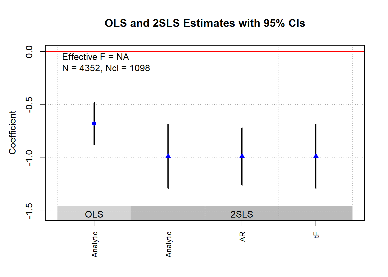
30.3.2 tF Procedure
Lee et al. (2022) propose a new method that is aligned better with traditional econometric training than AR, where it is called the tF procedure. It incorporates both the 1st-stage F-stat and the 2SLS \(t\)-value. This method is applicable to single instrumental variable (i.e., just-identified model), including
Randomized trials with imperfect compliance (G. W. Imbens and Angrist 1994).
Fuzzy Regression Discontinuity designs (Lee and Lemieux 2010).
Fuzzy regression kink designs (Card et al. 2015).
See I. Andrews, Stock, and Sun (2019) for a comparison between AR approach and tF Procedure.
tF Procedure:
Adjusts the t-ratio based on the first-stage F-statistic.
Rather than a fixed pretesting threshold, it applies an adjustment factor to 2SLS standard errors.
Adjustment factors are provided for 95% and 99% confidence levels.
Advantages of the tF Procedure:
Smooth Adjustment:
Gives usable finite confidence intervals for smaller F statistic values.
95% confidence is applicable for \(F > 3.84\), aligning with AR’s bounded 95% confidence intervals.
Clear Confidence Levels:
These levels incorporate effects of basing inference on the first-stage F.
Mirrors AR or other zero distortion procedures.
Robustness:
Robust against common error structures (e.g., heteroskedasticity or clustering and/or autocorrelated errors).
No further adjustments are necessary as long as robust variance estimators are consistently used (same robust variance estimator used for the 1st-stage as for the IV estimate).
Comparison to AR:
- Surprisingly, with \(F > 3.84\), AR’s expected interval length is infinite, while tF’s is finite (i.e., better).
Applicability:
The tF adjustment can re-evaluate published studies if the first-stage F-statistic is available.
Original data access is not needed.
Impacts in Applied Research:
Lee et al. (2022) examined recent single-instrument specification studies from the American Economic Review (AER).
Observations:
For at least 25% of the studied specifications, using tF increased confidence interval lengths by:
49% (5% significance level).
136% (1% significance level).
For specifications with \(F > 10\) and \(t > 1.96\), about 25% became statistically insignificant at the 5% level when adjusted using tF.
Conclusion: tF adjustments could greatly influence inferences in research employing t-ratio inferences.
Notation
- \(Y = X \beta + W \gamma + u\)
- \(X = Z \pi + W \xi + \nu\)
where
- \(W\): Additional covariates, possibly including an intercept term.
- \(X\): variable of interest
- \(Z\): instruments
Key Statistics:
\(t\)-ratio for the instrumental variable estimator: \(\hat{t} = \frac{\hat{\beta} - \beta_0}{\sqrt{\hat{V}_N (\hat{\beta})}}\)
\(t\)-ratio for the first-stage coefficient: \(\hat{f} = \frac{\hat{\pi}}{\sqrt{\hat{V}_N (\hat{\pi})}}\)
\(\hat{F} = \hat{f}^2\)
where
- \(\hat{\beta}\): Instrumental variable estimator.
- \(\hat{V}_N (\hat{\beta})\): Estimated variance of \(\hat{\beta}\), possibly robust to deal with non-iid errors.
- \(\hat{t}\): \(t\)-ratio under the null hypothesis.
- \(\hat{f}\): \(t\)-ratio under the null hypothesis of \(\pi=0\).
Traditional \(t\) Inference:
- In large samples, \(\hat{t}^2 \to^d t^2\)
- Standard normal critical values are \(\pm 1.96\) for 5% significance level testing.
Distortions in Inference in the case of IV:
- Use of a standard normal can lead to distorted inferences even in large samples.
- Despite large samples, t-distribution might not be normal.
- But magnitude of this distortion can be quantified.
- J. H. Stock and Yogo (2005) provides a formula for Wald test statistics using 2SLS.
- \(t^2\) formula allows for quantification of inference distortions.
- In the just-identified case with one endogenous regressor \(t^2 = f + t_{AR} + \rho f t_{AR}\) (J. H. Stock and Yogo 2005)
- \(\hat{f} \to^d f\) and \(\bar{f} = \frac{\pi}{\sqrt{\frac{1}{N} AV(\hat{\pi})}}\) and \(AV(\hat{\pi})\) is the asymptotic variance of \(\hat{\pi}\)
- \(t_{AR}\) is a standard normal with \(AR = t^2_{AR}\)
- \(\rho\) (degree of endogeneity) is the correlation of \(Zu\) and \(Z \nu\) (when data are homoskedastic, \(\rho\) is the correlation between \(u\) and \(\nu\))
Implications of \(t^2\) formula:
- Varies rejection rates depending on \(\rho\) value.
- \(\rho \in (0,0.5]\) (low) the t-ratio rejects at a probability below the nominal \(0.05\) rate
- \(\rho = 0.8\) (high) the rejection rate can be \(0.13\)
- In short, incorrect test size when relying solely on \(t^2\) (based on traditional econometric understanding)
To correct for this, one can
- Estimate the usually 2SLS standard errors
- Multiply the SE by the adjustment factor based on the observed first-stage \(\hat{F}\) stat
- One can go back to the traditional hypothesis by using either the t-ratio of confidence intervals
Lee et al. (2022) call this adjusted SE as “0.05 tF SE”.
library(ivDiag)
g <- ivDiag::ivDiag(
    data = rueda,
    Y = "e_vote_buying",
    D = "lm_pob_mesa",
    Z = "lz_pob_mesa_f",
    controls = c("lpopulation", "lpotencial"),
    cl = "muni_code",
    cores = 4,
    bootstrap = FALSE
)
g$tF
#>         F        cF      Coef        SE         t    CI2.5%   CI97.5%   p-value
#> 8598.3264    1.9600   -0.9835    0.1540   -6.3872   -1.2853   -0.6817    0.0000
# example in fixest package
library(fixest)
library(tidyverse)
base = iris
names(base) = c("y", "x1", "x_endo_1", "x_inst_1", "fe")
set.seed(2)
base$x_inst_2 = 0.2 * base$y + 0.2 * base$x_endo_1 + rnorm(150, sd = 0.5)
base$x_endo_2 = 0.2 * base$y - 0.2 * base$x_inst_1 + rnorm(150, sd = 0.5)
est_iv = feols(y ~ x1 | x_endo_1 + x_endo_2 ~ x_inst_1 + x_inst_2, base)
est_iv
#> TSLS estimation - Dep. Var.: y
#> Endo. : x_endo_1, x_endo_2
#> Instr. : x_inst_1, x_inst_2
#> Second stage: Dep. Var.: y
#> Observations: 150
#> Standard-errors: IID
#> Estimate Std. Error t value Pr(>|t|)
#> (Intercept) 1.831380 0.411435 4.45121 1.6844e-05 ***
#> fit_x_endo_1 0.444982 0.022086 20.14744 < 2.2e-16 ***
#> fit_x_endo_2 0.639916 0.307376 2.08186 3.9100e-02 *
#> x1 0.565095 0.084715 6.67051 4.9180e-10 ***
#> ---
#> Signif. codes: 0 '***' 0.001 '**' 0.01 '*' 0.05 '.' 0.1 ' ' 1
#> RMSE: 0.398842 Adj. R2: 0.761653
#> F-test (1st stage), x_endo_1: stat = 903.2 , p < 2.2e-16 , on 2 and 146 DoF.
#> F-test (1st stage), x_endo_2: stat = 3.25828, p = 0.041268, on 2 and 146 DoF.
#> Wu-Hausman: stat = 6.79183, p = 0.001518, on 2 and 144 DoF.
res_est_iv <- est_iv$coeftable |>
rownames_to_column()
coef_of_interest <-
res_est_iv[res_est_iv$rowname == "fit_x_endo_1", "Estimate"]
se_of_interest <-
res_est_iv[res_est_iv$rowname == "fit_x_endo_1", "Std. Error"]
fstat_1st <- fitstat(est_iv, type = "ivf1")[[1]]$stat
# To get the correct SE based on 1st-stage F-stat (This result is similar without adjustment since F is large)
# the results are the new CIS and p.value
tF(coef = coef_of_interest, se = se_of_interest, Fstat = fstat_1st) |>
causalverse::nice_tab(5)
#> F cF Coef SE t CI2.5. CI97.5. p.value
#> 1 903.1628 1.96 0.44498 0.02209 20.14744 0.40169 0.48827 0
# We can try to see a different 1st-stage F-stat and how it changes the results
tF(coef = coef_of_interest, se = se_of_interest, Fstat = 2) |>
causalverse::nice_tab(5)
#> F cF Coef SE t CI2.5. CI97.5. p.value
#> 1 2 18.66 0.44498 0.02209 20.14744 0.03285 0.85711 0.03432