6.1 Inference

Since \(Y_i = f(\mathbf{x}_i,\theta) + \epsilon_i\), where \(\epsilon_i \sim iid(0,\sigma^2)\), we can obtain \(\hat{\theta}\) by minimizing \(\sum_{i=1}^{n}(Y_i - f(x_i,\theta))^2\) and estimate \(s^2 = \hat{\sigma}^2_{\epsilon}=\frac{\sum_{i=1}^{n}(Y_i - f(x_i,\theta))^2}{n-p}\)

6.1.1 Linear Function of the Parameters

If we assume \(\epsilon_i \sim N(0,\sigma^2)\), then

\[ \hat{\theta} \sim AN(\mathbf{\theta},\sigma^2[\mathbf{F}(\theta)'\mathbf{F}(\theta)]^{-1}) \]

where AN = asymptotic normality

Asymptotic means we have enough data to make inference (As your sample size increases, this becomes more and more accurate (to the true value)).

Since we want to do inference on linear combinations of parameters or contrasts.

If we have \(\mathbf{\theta} = (\theta_0,\theta_1,\theta_2)'\) and we want to look at \(\theta_1 - \theta_2\); we can define vector \(\mathbf{a} = (0,1,-1)'\), consider inference for \(\mathbf{a'\theta}\)

Rules for expectation and variance of a fixed vector \(\mathbf{a}\) and random vector \(\mathbf{Z}\);

\[ \begin{aligned} E(\mathbf{a'Z}) &= \mathbf{a'}E(\mathbf{Z}) \\ var(\mathbf{a'Z}) &= \mathbf{a'}var(\mathbf{Z}) \mathbf{a} \end{aligned} \]

Then,

\[ \mathbf{a'\hat{\theta}} \sim AN(\mathbf{a'\theta},\sigma^2\mathbf{a'[F(\theta)'F(\theta)]^{-1}a}) \]

and \(\mathbf{a'\hat{\theta}}\) is asymptotically independent of \(s^2\) (to order 1/n) then

\[ \frac{\mathbf{a'\hat{\theta}-a'\theta}}{s(\mathbf{a'[F(\theta)'F(\theta)]^{-1}a})^{1/2}} \sim t_{n-p} \]

to construct \(100(1-\alpha)\%\) confidence interval for \(\mathbf{a'\theta}\)

\[ \mathbf{a'\theta} \pm t_{(1-\alpha/2,n-p)}s(\mathbf{a'[F(\theta)'F(\theta)]^{-1}a})^{1/2} \]

Suppose \(\mathbf{a'} = (0,...,j,...,0)\). Then, a confidence interval for the \(j\)-th element of \(\mathbf{\theta}\) is

\[ \hat{\theta}_j \pm t_{(1-\alpha/2,n-p)}s\sqrt{\hat{c}^{j}} \]

where \(\hat{c}^{j}\) is the \(j\)-th diagonal element of \([\mathbf{F(\hat{\theta})'F(\hat{\theta})}]^{-1}\)

#set a seed value
set.seed(23)

#Generate x as 100 integers using seq function
x <- seq(0, 100, 1)

#Generate y as a*e^(bx)+c
y <- runif(1, 0, 20) * exp(runif(1, 0.005, 0.075) * x) + runif(101, 0, 5)

# visualize
plot(x, y)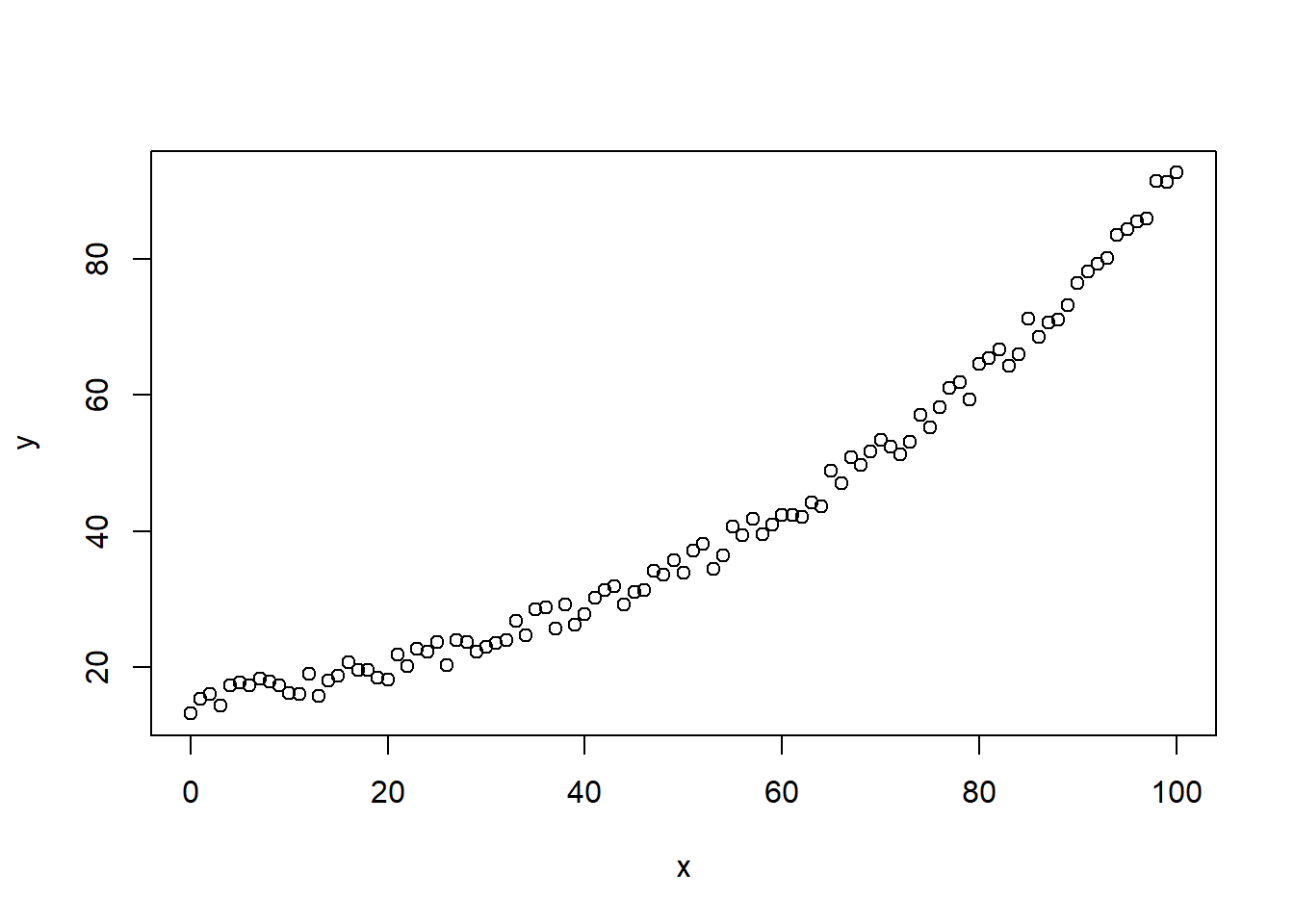

#define our data frame
datf = data.frame(x, y)

#define our model function
mod = function(a, b, x)
    a * exp(b * x)

In this example, we can get the starting values by using linearized version of the function \(\log y = \log a + b x\). Then, we can fit a linear regression to this and use our estimates as starting values

#get starting values by linearizing
lin_mod = lm(log(y) ~ x, data = datf)

#convert the a parameter back from the log scale; b is ok
astrt = exp(as.numeric(lin_mod$coef[1]))
bstrt = as.numeric(lin_mod$coef[2])
print(c(astrt, bstrt))
#> [1] 14.07964761  0.01855635

with nls, we can fit the nonlinear model via least squares

nlin_mod = nls(y ~ mod(a, b, x),
               start = list(a = astrt, b = bstrt),
               data = datf)

#look at model fit summary
summary(nlin_mod)
#> 
#> Formula: y ~ mod(a, b, x)
#> 
#> Parameters:
#>    Estimate Std. Error t value Pr(>|t|)    
#> a 13.603909   0.165390   82.25   <2e-16 ***
#> b  0.019110   0.000153  124.90   <2e-16 ***
#> ---
#> Signif. codes:  0 '***' 0.001 '**' 0.01 '*' 0.05 '.' 0.1 ' ' 1
#> 
#> Residual standard error: 1.542 on 99 degrees of freedom
#> 
#> Number of iterations to convergence: 3 
#> Achieved convergence tolerance: 7.006e-07

#add prediction to plot
plot(x, y)
lines(x, predict(nlin_mod), col = "red")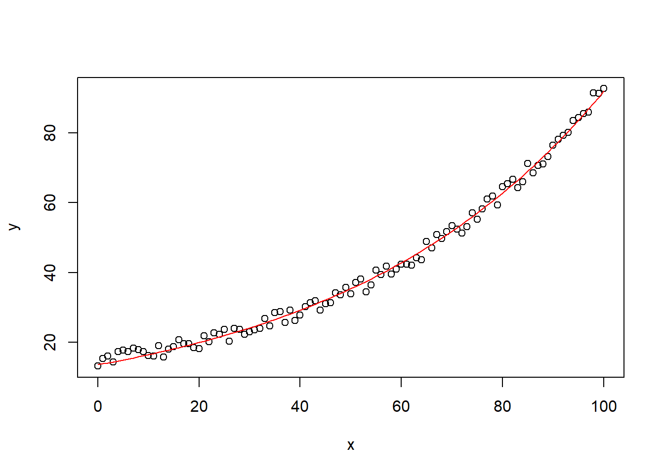

6.1.2 Nonlinear

Suppose that \(h(\theta)\) is a nonlinear function of the parameters. We can use Taylor series about \(\theta\)

\[ h(\hat{\theta}) \approx h(\theta) + \mathbf{h}'[\hat{\theta}-\theta] \]

where \(\mathbf{h} = (\frac{\partial h}{\partial \theta_1},...,\frac{\partial h}{\partial \theta_p})'\)

with

\[ \begin{aligned} E( \hat{\theta}) &\approx \theta \\ var(\hat{\theta}) &\approx \sigma^2[\mathbf{F(\theta)'F(\theta)}]^{-1} \\ E(h(\hat{\theta})) &\approx h(\theta) \\ var(h(\hat{\theta})) &\approx \sigma^2 \mathbf{h'[F(\theta)'F(\theta)]^{-1}h} \end{aligned} \]

Thus,

\[ h(\hat{\theta}) \sim AN(h(\theta),\sigma^2\mathbf{h'[F(\theta)'F(\theta)]^{-1}h}) \]

and an approximate \(100(1-\alpha)\%\) confidence interval for \(h(\theta)\) is

\[ h(\hat{\theta}) \pm t_{(1-\alpha/2;n-p)}s(\mathbf{h'[F(\theta)'F(\theta)]^{-1}h})^{1/2} \]

where \(\mathbf{h}\) and \(\mathbf{F}(\theta)\) are evaluated at \(\hat{\theta}\)

Regarding prediction interval for Y at \(x=x_0\)

\[ \begin{aligned} Y_0 &= f(x_0;\theta) + \epsilon_0, \epsilon_0 \sim N(0,\sigma^2) \\ \hat{Y}_0 &= f(x_0,\hat{\theta}) \end{aligned} \]

As \(n \to \infty\), \(\hat{\theta} \to \theta\), so we

\[ f(x_0, \hat{\theta}) \approx f(x_0,\theta) + \mathbf{f}_0(\mathbf{\theta})'[\hat{\theta}-\theta] \]

where

\[ f_0(\theta)= (\frac{\partial f(x_0,\theta)}{\partial \theta_1},..,\frac{\partial f(x_0,\theta)}{\partial \theta_p})' \]

(note: this \(f_0(\theta)\) is different from \(f(\theta)\)).

\[ \begin{aligned} Y_0 - \hat{Y}_0 &\approx Y_0 - f(x_0,\theta) - f_0(\theta)'[\hat{\theta}-\theta] \\ &= \epsilon_0 - f_0(\theta)'[\hat{\theta}-\theta] \end{aligned} \]

\[ \begin{aligned} E(Y_0 - \hat{Y}_0) &\approx E(\epsilon_0)E(\hat{\theta}-\theta) = 0 \\ var(Y_0 - \hat{Y}_0) &\approx var(\epsilon_0 - \mathbf{(f_0(\theta)'[\hat{\theta}-\theta])}) \\ &= \sigma^2 + \sigma^2 \mathbf{f_0 (\theta)'[F(\theta)'F(\theta)]^{-1}f_0(\theta)} \\ &= \sigma^2 (1 + \mathbf{f_0 (\theta)'[F(\theta)'F(\theta)]^{-1}f_0(\theta)}) \end{aligned} \]

Hence, combining

\[ Y_0 - \hat{Y}_0 \sim AN (0,\sigma^2 (1 + \mathbf{f_0 (\theta)'[F(\theta)'F(\theta)]^{-1}f_0(\theta)})) \]

Note:

Confidence intervals for the mean response \(Y_i\) (which is different from prediction intervals) can be obtained similarly.