27.1 Application
27.1.1 ECIC package
library(ecic)
data(dat, package = "ecic")
mod =
  ecic(
    yvar  = lemp,         # dependent variable
    gvar  = first.treat,  # group indicator
    tvar  = year,         # time indicator
    ivar  = countyreal,   # unit ID
    dat   = dat,          # dataset
    boot  = "weighted",   # bootstrap proceduce ("no", "normal", or "weighted")
    nReps = 3            # number of bootstrap runs
    )
mod_res <- summary(mod)
mod_res
#>   perc    coefs          se
#> 1  0.1 1.206140 0.021351711
#> 2  0.2 1.316599 0.009225026
#> 3  0.3 1.449963 0.001859468
#> 4  0.4 1.583415 0.015296156
#> 5  0.5 1.739932 0.011240454
#> 6  0.6 1.915558 0.013060348
#> 7  0.7 2.114966 0.014482208
#> 8  0.8 2.363105 0.005173865
#> 9  0.9 2.779202 0.020831180

ecic_plot(mod_res)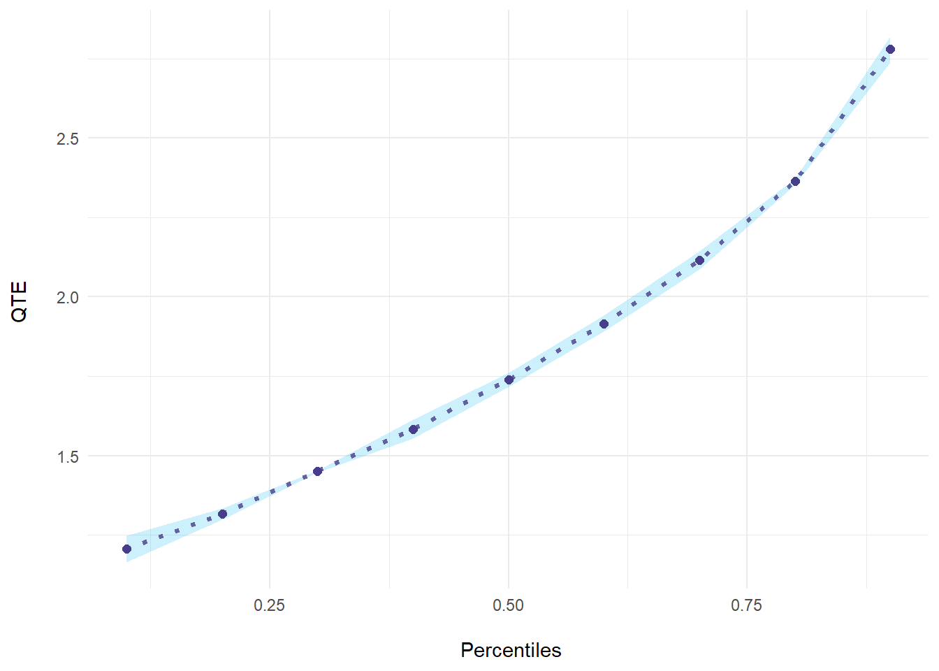
27.1.2 QTE package
library(qte)
data(lalonde)

# randomized setting
# qte is identical to qtet
jt.rand <-
    ci.qtet(
        re78 ~ treat,
        data = lalonde.exp,
        iters = 10
    )
summary(jt.rand)
#>
#> Quantile Treatment Effect:
#>
#> tau  QTE Std. Error
#> 0.05    0.00    0.00
#> 0.1     0.00    0.00
#> 0.15    0.00    0.00
#> 0.2     0.00   18.33
#> 0.25  338.65  377.74
#> 0.3   846.40  470.45
#> 0.35 1451.51  515.86
#> 0.4  1177.72  869.19
#> 0.45 1396.08  918.39
#> 0.5  1123.55  925.74
#> 0.55 1181.54  938.82
#> 0.6  1466.51  951.64
#> 0.65 2115.04  892.16
#> 0.7  1795.12  842.66
#> 0.75 2347.49  678.45
#> 0.8  2278.12  971.21
#> 0.85 2178.28  973.90
#> 0.9  3239.60 1889.23
#> 0.95 3979.62 2872.52
#>
#> Average Treatment Effect:    1794.34
#>   Std. Error:        665.59
ggqte(jt.rand)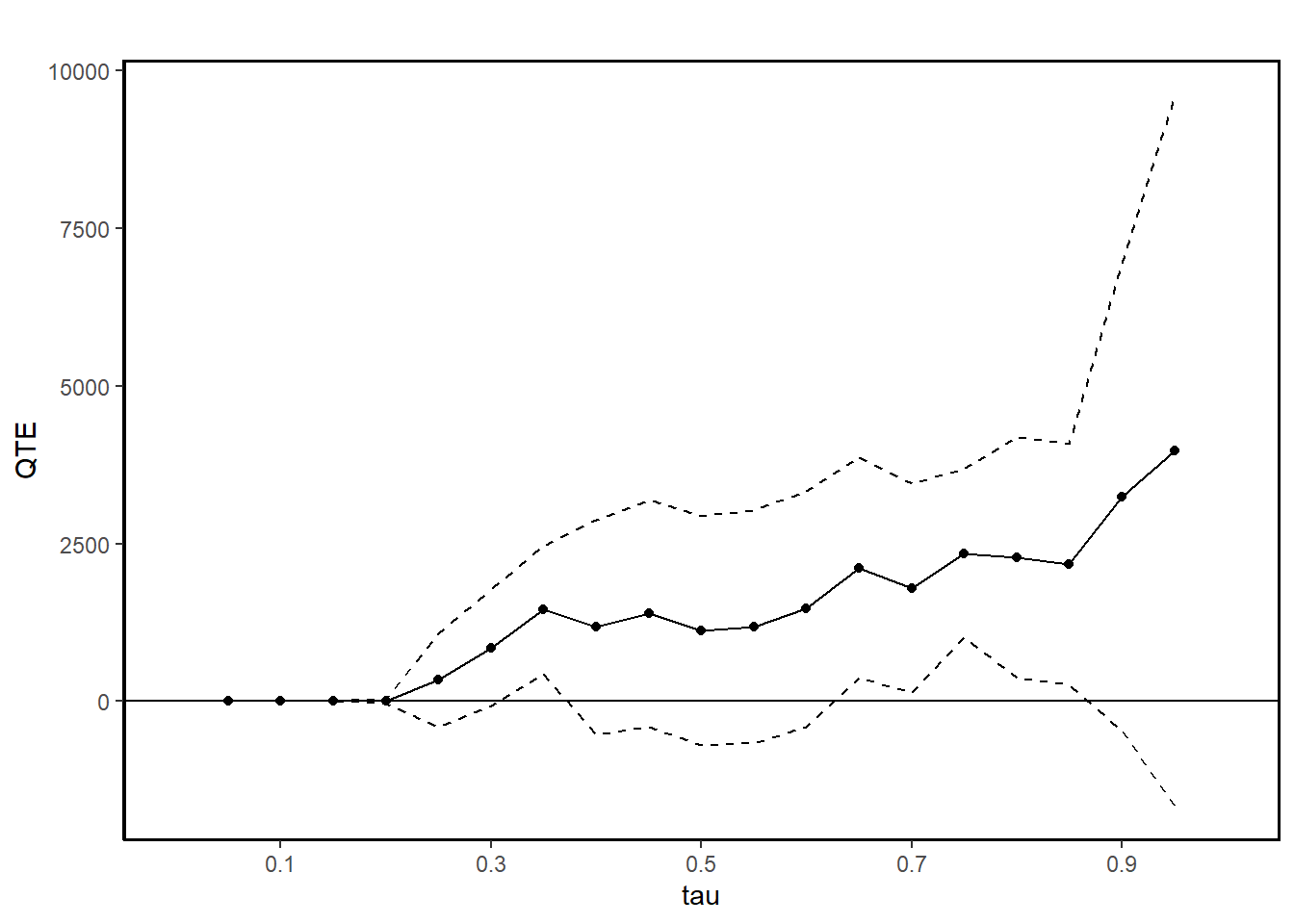
# conditional independence assumption (CIA)
jt.cia <- ci.qte(
    re78 ~ treat,
    xformla =  ~ age + education,
    data = lalonde.psid,
    iters = 10
)
summary(jt.cia)
#>
#> Quantile Treatment Effect:
#>
#> tau  QTE Std. Error
#> 0.05      0.00        0.00
#> 0.1       0.00        0.00
#> 0.15  -4433.18      710.76
#> 0.2   -8219.15      419.90
#> 0.25 -10435.74      793.20
#> 0.3  -12232.03     1037.03
#> 0.35 -12428.30     1425.39
#> 0.4  -14195.24     1793.20
#> 0.45 -14248.66     1907.98
#> 0.5  -15538.67     2095.11
#> 0.55 -16550.71     2329.67
#> 0.6  -15595.02     2686.45
#> 0.65 -15827.52     2745.62
#> 0.7  -16090.32     3390.26
#> 0.75 -16091.49     3376.67
#> 0.8  -17864.76     3245.52
#> 0.85 -16756.71     3533.91
#> 0.9  -17914.99     2305.10
#> 0.95 -23646.22     2003.55
#>
#> Average Treatment Effect:    -13435.40
#>   Std. Error:        1259.01
ggqte(jt.cia)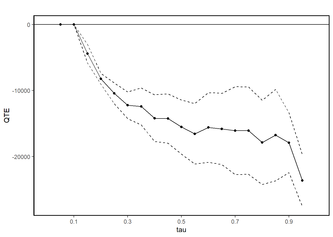
jt.ciat <- ci.qtet(
    re78 ~ treat,
    xformla =  ~ age + education,
    data = lalonde.psid,
    iters = 10
)
summary(jt.ciat)
#>
#> Quantile Treatment Effect:
#>
#> tau  QTE Std. Error
#> 0.05      0.00        0.00
#> 0.1   -1018.15      614.29
#> 0.15  -3251.00     1557.37
#> 0.2   -7240.86     1433.54
#> 0.25  -8379.94      475.33
#> 0.3   -8758.82      345.53
#> 0.35  -9897.44      606.54
#> 0.4  -10239.57      747.91
#> 0.45 -10751.39      736.39
#> 0.5  -10570.14      899.75
#> 0.55 -11348.96      898.80
#> 0.6  -11550.84      687.20
#> 0.65 -12203.56      780.92
#> 0.7  -13277.72      979.47
#> 0.75 -14011.74      993.28
#> 0.8  -14373.95      706.69
#> 0.85 -14499.18     1048.62
#> 0.9  -15008.63     2201.11
#> 0.95 -15954.05     2655.30
#>
#> Average Treatment Effect:    4266.19
#>   Std. Error:        600.51
ggqte(jt.ciat)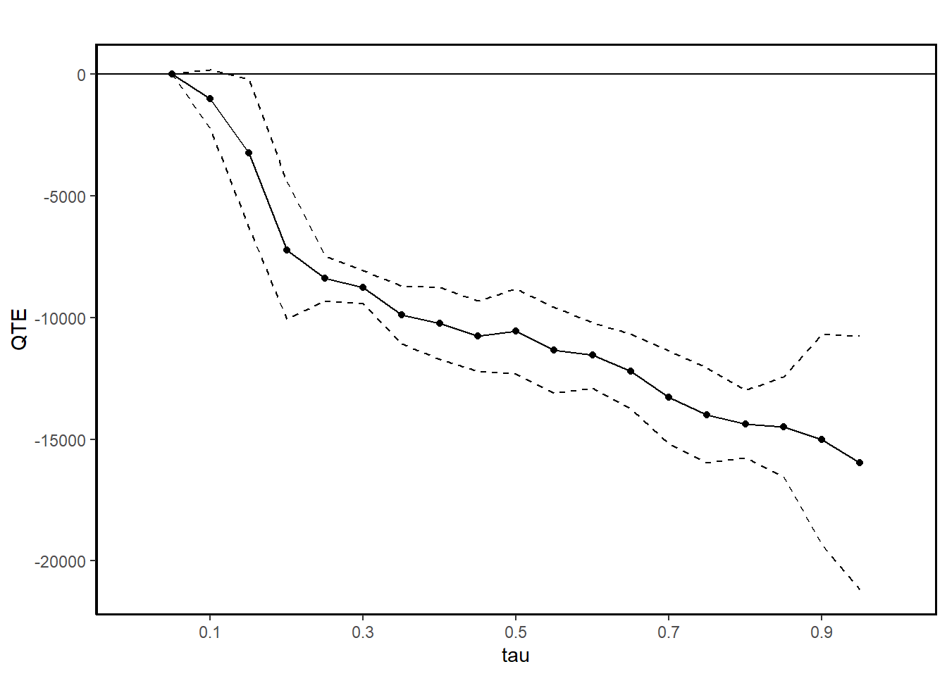
QTE compares quantiles of the entire population under treatment and control, whereas QTET compares quantiles within the treated group itself. This difference means that QTE reflects the overall population-level impact, while QTET focuses on the treated group’s specific impact.
CIA enables identification of both QTE and QTET, but since QTET is conditional on treatment, it might reflect different effects than QTE, especially when the treatment effect is heterogeneous across different subpopulations. For example, the QTE could show a more generalized effect across all individuals, while the QTET may reveal stronger or weaker effects for the subgroup that actually received the treatment.
These are DID-like models
- With the distributional difference-in-differences assumption Callaway and Li (2019), which is an extension of the parallel trends assumption, we can estimate QTET.
# distributional DiD assumption
jt.pqtet <- panel.qtet(
    re ~ treat,
    t = 1978,
    tmin1 = 1975,
    tmin2 = 1974,
    tname = "year",
    idname = "id",
    data = lalonde.psid.panel,
    iters = 10
)
summary(jt.pqtet)
#>
#> Quantile Treatment Effect:
#>
#> tau  QTE Std. Error
#> 0.05  4779.21     1222.37
#> 0.1   1987.35      776.82
#> 0.15   842.95     3332.09
#> 0.2  -7366.04     4852.87
#> 0.25 -8449.96     3522.70
#> 0.3  -7992.15     1201.51
#> 0.35 -7429.21     1161.43
#> 0.4  -6597.37     1288.64
#> 0.45 -5519.45     1391.04
#> 0.5  -4702.88     1129.80
#> 0.55 -3904.52     1131.23
#> 0.6  -2741.80     1157.60
#> 0.65 -1507.31     1223.03
#> 0.7   -771.12     1264.45
#> 0.75   707.81     1280.34
#> 0.8    580.00      793.09
#> 0.85   821.75      969.38
#> 0.9   -250.77     1662.49
#> 0.95 -1874.54     2706.67
#>
#> Average Treatment Effect:    2326.51
#>   Std. Error:        795.44
ggqte(jt.pqtet)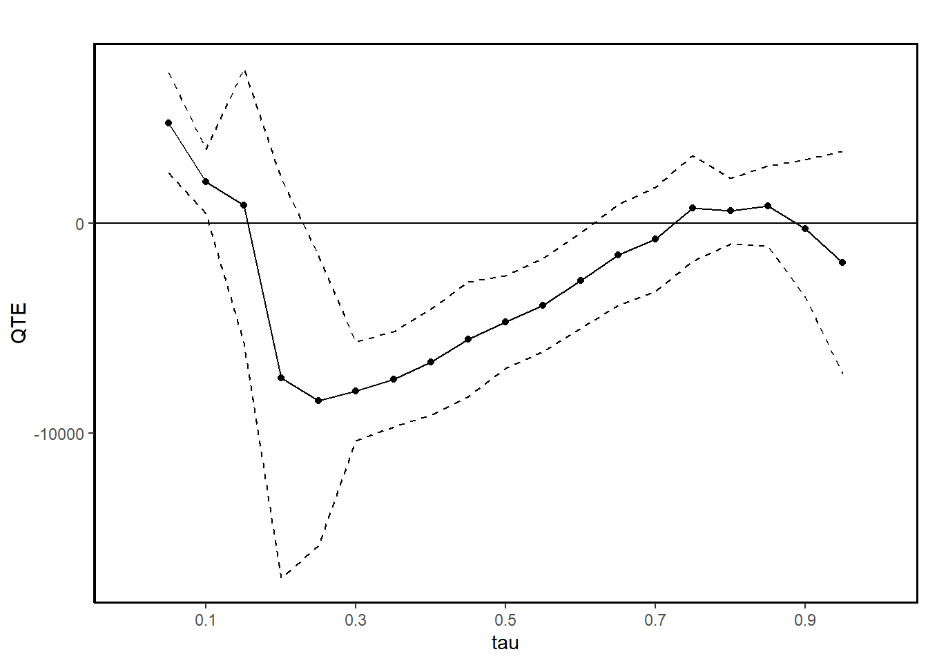
- With 2 periods, the distributional DiD assumption can partially identify QTET with bounds (Fan and Yu 2012)
res_bound <-
    bounds(
        re ~ treat,
        t = 1978,
        tmin1 = 1975,
        data = lalonde.psid.panel,
        idname = "id",
        tname = "year"
    )
summary(res_bound)
#>
#> Bounds on the Quantile Treatment Effect on the Treated:
#>
#> tau  Lower Bound Upper Bound
#>         tau  Lower Bound Upper Bound
#>        0.05       -51.72           0
#>         0.1     -1220.84           0
#>        0.15      -1881.9           0
#>         0.2     -2601.32           0
#>        0.25     -2916.38      485.23
#>         0.3     -3080.16      943.05
#>        0.35     -3327.89     1505.98
#>         0.4     -3240.59     2133.59
#>        0.45     -2982.51     2616.84
#>         0.5     -3108.01      2566.2
#>        0.55     -3342.66     2672.82
#>         0.6      -3491.4      3065.7
#>        0.65     -3739.74     3349.74
#>         0.7     -4647.82     2992.03
#>        0.75     -4826.78     3219.32
#>         0.8      -5801.7     2702.33
#>        0.85     -6588.61     2499.41
#>         0.9     -8953.84     2020.84
#>        0.95    -14283.61      397.04
#>
#> Average Treatment Effect on the Treated: 2326.51
plot(res_bound)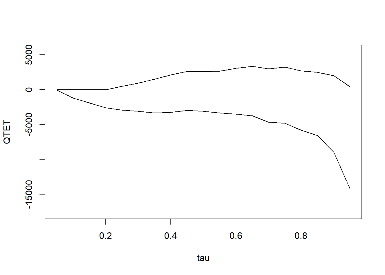
- With a restrictive assumption that difference in the quantiles of the distribution of potential outcomes for the treated and untreated groups be the same for all values of quantiles, we can have the mean DiD model
jt.mdid <- ddid2(
    re ~ treat,
    t = 1978,
    tmin1 = 1975,
    tname = "year",
    idname = "id",
    data = lalonde.psid.panel,
    iters = 10
)
summary(jt.mdid)
#>
#> Quantile Treatment Effect:
#>
#> tau  QTE Std. Error
#> 0.05 10616.61      744.99
#> 0.1   5019.83      447.82
#> 0.15  2388.12      334.57
#> 0.2   1033.23      365.01
#> 0.25   485.23      445.95
#> 0.3    943.05      631.10
#> 0.35   931.45      756.72
#> 0.4    945.35      888.69
#> 0.45  1205.88      903.88
#> 0.5   1362.11      778.89
#> 0.55  1279.05      871.73
#> 0.6   1618.13      734.08
#> 0.65  1834.30      674.83
#> 0.7   1326.06      793.46
#> 0.75  1586.35      714.42
#> 0.8   1256.09      591.37
#> 0.85   723.10      871.86
#> 0.9    251.36     1703.13
#> 0.95 -1509.92     2033.88
#>
#> Average Treatment Effect:    2326.51
#>   Std. Error:        514.81
plot(jt.mdid)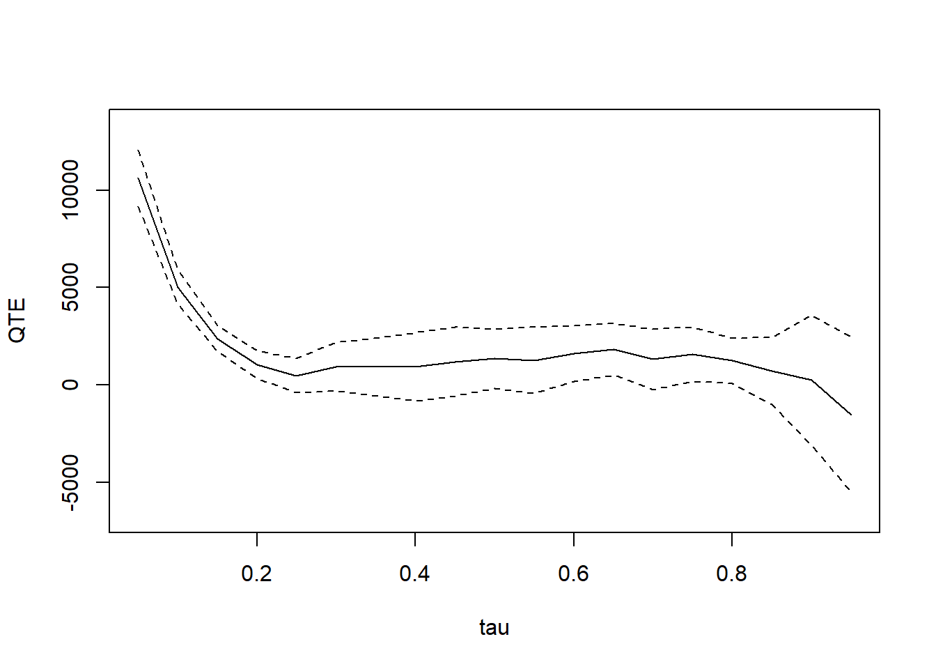
On top of the distributional DiD assumption, we need copula stability assumption (i.e., If, before the treatment, the units with the highest outcomes were improving the most, we would expect to see them improving the most in the current period too.) for these models:
| Aspect | QDiD | CiC |
|---|---|---|
| Treatment of Time and Group | Symmetric | Asymmetric |
| QTET Computation | Not inherently scale-invariant | Outcome Variable Scale-Invariant |