12.4 Panel Data
Detail notes in R can be found here
Follows an individual over T time periods.
Panel data structure is like having n samples of time series data
Characteristics
Information both across individuals and over time (cross-sectional and time-series)
N individuals and T time periods
Data can be either
- Balanced: all individuals are observed in all time periods
- Unbalanced: all individuals are not observed in all time periods.
Assume correlation (clustering) over time for a given individual, with independence over individuals.
Types
- Short panel: many individuals and few time periods.
- Long panel: many time periods and few individuals
- Both: many time periods and many individuals
Time Trends and Time Effects
- Nonlinear
- Seasonality
- Discontinuous shocks
Regressors
- Time-invariant regressors xit=xi for all t (e.g., gender, race, education) have zero within variation
- Individual-invariant regressors xit=xt for all i (e.g., time trend, economy trends) have zero between variation
Variation for the dependent variable and regressors
- Overall variation: variation over time and individuals.
- Between variation: variation between individuals
- Within variation: variation within individuals (over time).
| Estimate | Formula |
|---|---|
| Individual mean | ¯xi=1T∑txit |
| Overall mean | ˉx=1NT∑i∑txit |
| Overall Variance | s2O=1NT−1∑i∑t(xit−ˉx)2 |
| Between variance | s2B=1N−1∑i(¯xi−ˉx)2 |
| Within variance | s2W=1NT−1∑i∑t(xit−¯xi)2=1NT−1∑i∑t(xit−¯xi+ˉx)2 |
Note: s2O≈s2B+s2W
Since we have n observation for each time period t, we can control for each time effect separately by including time dummies (time effects)
yit=xitβ+d1δ1+...+dT−1δT−1+ϵit
Note: we cannot use these many time dummies in time series data because in time series data, our n is 1. Hence, there is no variation, and sometimes not enough data compared to variables to estimate coefficients.
Unobserved Effects Model Similar to group clustering, assume that there is a random effect that captures differences across individuals but is constant in time.
yit=xitβ+d1δ1+...+dT−1δT−1+ci+uit
where
- ci+uit=ϵit
- ci unobserved individual heterogeneity (effect)
- uit idiosyncratic shock
- ϵit unobserved error term.
12.4.1 Pooled OLS Estimator
If ci is uncorrelated with xit
E(x′it(ci+uit))=0
then [A3a] still holds. And we have Pooled OLS consistent.
If A4 does not hold, OLS is still consistent, but not efficient, and we need cluster robust SE.
Sufficient for [A3a] to hold, we need
- Exogeneity for uit [A3a] (contemporaneous exogeneity): E(x′ituit)=0 time varying error
- Random Effect Assumption (time constant error): E(x′itci)=0
Pooled OLS will give you consistent coefficient estimates under A1, A2, [A3a] (for both uit and RE assumption), and A5 (randomly sampling across i).
12.4.2 Individual-specific effects model
- If we believe that there is unobserved heterogeneity across individual (e.g., unobserved ability of an individual affects y), If the individual-specific effects are correlated with the regressors, then we have the Fixed Effects Estimator. and if they are not correlated we have the Random Effects Estimator.
12.4.2.1 Random Effects Estimator
Random Effects estimator is the Feasible GLS estimator that assumes uit is serially uncorrelated and homoskedastic
12.4.2.2 Fixed Effects Estimator
also known as Within Estimator uses within variation (over time)
If the RE assumption is not hold (E(x′itci)≠0), then A3a does not hold (E(x′itϵi)≠0).
Hence, the OLS and RE are inconsistent/biased (because of omitted variable bias)
However, FE can only fix bias due to time-invariant factors (both observables and unobservables) correlated with treatment (not time-variant factors that correlated with the treatment).
The traditional FE technique is flawed when lagged dependent variables are included in the model. (Nickell 1981) (Narayanan and Nair 2013)
With measurement error in the independent, FE will exacerbate the errors-in-the-variables bias.
12.4.2.2.1 Demean Approach
To deal with violation in ci, we have
yit=xitβ+ci+uit
¯yi=¯xiβ+ci+¯ui
where the second equation is the time averaged equation
using within transformation, we have
yit−¯yi=(xit−¯xi)β+uit−¯ui
because ci is time constant.
The Fixed Effects estimator uses POLS on the transformed equation
yit−¯yi=(xit−¯xi)β+d1δ1+...+dT−2δT−2+uit−¯ui
we need A3 (strict exogeneity) (E((xit−¯xi)′(uit−¯ui)=0) to have FE consistent.
Variables that are time constant will be absorbed into ci. Hence we cannot make inference on time constant independent variables.
- If you are interested in the effects of time-invariant variables, you could consider the OLS or between estimator
It’s recommended that you should still use cluster robust standard errors.
12.4.2.2.2 Dummy Approach
Equivalent to the within transformation (i.e., mathematically equivalent to Demean Approach), we can have the fixed effect estimator be the same with the dummy regression
yit=xitβ+d1δ1+...+dT−2δT−2+c1γ1+...+cn−1γn−1+uit
where
ci={1if observation is i0otherwise
- The standard error is incorrectly calculated.
- the FE within transformation is controlling for any difference across individual which is allowed to correlated with observables.
12.4.2.2.3 First-difference Approach
Economists typically use this approach
yit−yi(t−1)=(xit−xi(t−1))β++(uit−ui(t−1))
12.4.2.2.4 Fixed Effects Summary
The three approaches are almost equivalent.
Demean Approach is mathematically equivalent to Dummy Approach
If you have only 1 period, all 3 are the same.
Since fixed effect is a within estimator, only status changes can contribute to β variation.
- Hence, with a small number of changes then the standard error for β will explode
Status changes mean subjects change from (1) control to treatment group or (2) treatment to control group. Those who have status change, we call them switchers.
Treatment effect is typically non-directional.
You can give a parameter for the direction if needed.
Issues:
You could have fundamental difference between switchers and non-switchers. Even though we can’t definitive test this, but providing descriptive statistics on switchers and non-switchers can give us confidence in our conclusion.
Because fixed effects focus on bias reduction, you might have larger variance (typically, with fixed effects you will have less df)
If the true model is random effect, economists typically don’t care, especially when ci is the random effect and ci⊥xit (because RE assumption is that it is unrelated to xit). The reason why economists don’t care is because RE wouldn’t correct bias, it only improves efficiency over OLS.
You can estimate FE for different units (not just individuals).
FE removes bias from time invariant factors but not without costs because it uses within variation, which imposes strict exogeneity assumption on uit: E[(xit−ˉxi)(uit−ˉuit)]=0
Recall
Yit=β0+Xitβ1+αi+uit
where ϵit=αi+uit
ˆσ2ϵ=SSROLSNT−K
ˆσ2u=SSRFENT−(N+K)=SSRFEN(T−1)−K
It’s ambiguous whether your variance of error changes up or down because SSR can increase while the denominator decreases.
FE can be unbiased, but not consistent (i.e., not converging to the true effect)
12.4.2.2.6 Blau (1999)
Intergenerational mobility
If we transfer resources to low income family, can we generate upward mobility (increase ability)?
Mechanisms for intergenerational mobility
- Genetic (policy can’t affect) (i.e., ability endowment)
- Environmental indirect
- Environmental direct
%ΔHuman capital%Δincome
- Financial transfer
Income measures:
- Total household income
- Wage income
- Non-wage income
- Annual versus permanent income
Core control variables:
Bad controls are those jointly determined with dependent variable
Control by mother = choice by mother
Uncontrolled by mothers:
mother race
location of birth
education of parents
household structure at age 14
Yijt=Xjtβi+Ijtαi+ϵijt
where
i = test
j = individual (child)
t = time
Grandmother’s model
Since child is nested within mother and mother nested within grandmother, the fixed effect of child is included in the fixed effect of mother, which is included in the fixed-effect of grandmother
Yijgmt=Xitβi+Ijtαi+γg+uijgmt
where
i = test, j = kid, m = mother, g = grandmother
where γg includes γm includes γj
Grandma fixed-effect
Pros:
control for some genetics + fixed characteristics of how mother are raised
can estimate effect of parameter income
Con:
- Might not be a sufficient control
Common to cluster a the fixed-effect level (common correlated component)
Fixed effect exaggerates attenuation bias
Error rate on survey can help you fix this (plug in the number only , but not the uncertainty associated with that number).
12.4.2.2.7 Babcock (2010)
Tijct=α0+Sjctα1+Xijctα2+uijct
where
Sjct is the average class expectation
Xijctα2 is the individual characteristics
i student
j instructor
c course
t time
Tijct=β0+Sjctβ1+Xijctβ2+μjc+ϵijct
where μjc is instructor by course fixed effect (unique id), which is different from (θj+δc)
- Decrease course shopping because conditioned on available information (μjc) (class grade and instructor’s info).
- Grade expectation change even though class materials stay the same
Identification strategy is
- Under (fixed) time-varying factor that could bias my coefficient (simultaneity)
Yijt=Xitβ1+Teacher Experiencejtβ2+Teacher educationjtβ3+Teacher scoreitβ4+⋯+ϵijt
Drop teacher characteristics, and include teacher dummy effect
Yijt=Xitα+Γitθj+uijt
where α is the within teacher (conditional on teacher fixed effect) and j=1→(J−1)
Nuisance in the sense that we don’t about the interpretation of α
The least we can say about θj is the teacher effect conditional on student test score.
Yijt=Xitγ+ϵijt
γ is between within (unconditional) and eijt is the prediction error
eijt=Titδj+˜eijt
where δj is the mean for each group
Yijkt=Yijkt−1+Xitβ+Titτj+(Wi+Pk+ϵijkt)
where
Yijkt−1 = lag control
τj = teacher fixed time
Wi is the student fixed effect
Pk is the school fixed effect
uijkt=Wi+Pk+ϵijkt
And we worry about selection on class and school
Bias in τ (for 1 teacher) is
1NjN∑i=1(Wi+Pk+ϵijkt)
where Nj = the number of student in class with teacher j
then we can Pk+1Nj∑Nji=1(Wi+ϵijkt)
Shocks from small class can bias τ
1NjNj∑i=1ϵijkt≠0
which will inflate the teacher fixed effect
Even if we create random teacher fixed effect and put it in the model, it still contains bias mentioned above which can still τ (but we do not know the way it will affect - whether more positive or negative).
If teachers switch schools, then we can estimate both teacher and school fixed effect (mobility web thin vs. thick)
Mobility web refers to the web of switchers (i.e., from one status to another).
Yijkt=Yijk(t−1)α+Xitβ+Titτ+Pk+ϵijkt
If we demean (fixed-effect), τ (teacher fixed effect) will go away
If you want to examine teacher fixed effect, we have to include teacher fixed effect
Control for school, the article argues that there is no selection bias
For 1Nj∑Nji=1ϵijkt (teacher-level average residuals), var(τ) does not change with Nj (Figure 2 in the paper). In words, the quality of teachers is not a function of the number of students
If var(τ)=0 it means that teacher quality does not matter
Spin-off of Measurement Error: Sampling error or estimation error
ˆτj=τj+λj
var(ˆτ)=var(τ+λ)
Assume cov(τj,λj)=0 (reasonable) In words, your randomness in getting children does not correlation with teacher quality.
Hence,
var(ˆτ)=var(τ)+var(λ)var(τ)=var(ˆτ)−var(λ)
We have var(ˆτ) and we need to estimate var(λ)
var(λ)=1JJ∑j=1ˆσ2j where ˆσ2j is the squared standard error of the teacher j (a function of n)
Hence,
var(τ)var(ˆτ)=reliability=true variance signal also known as how much noise in ˆτ and
1−var(τ)var(ˆτ)=noise
Even in cases where the true relationship is that τ is a function of Nj, then our recovery method for λ is still not affected
To examine our assumption
ˆτj=β0+Xjβ1+ϵj
Regressing teacher fixed-effect on teacher characteristics should give us R2 close to 0, because teacher characteristics cannot predict sampling error (ˆτ contain sampling error)
12.4.3 Tests for Assumptions
We typically don’t test heteroskedasticity because we will use robust covariance matrix estimation anyway.
Dataset
library("plm")
data("EmplUK", package="plm")
data("Produc", package="plm")
data("Grunfeld", package="plm")
data("Wages", package="plm")
12.4.3.1 Poolability
also known as an F test of stability (or Chow test) for the coefficients
H0: All individuals have the same coefficients (i.e., equal coefficients for all individuals).
Ha Different individuals have different coefficients.
Notes:
- Under a within (i.e., fixed) model, different intercepts for each individual are assumed
- Under random model, same intercept is assumed
library(plm)
plm::pooltest(inv~value+capital, data=Grunfeld, model="within")
#>
#>  F statistic
#>
#> data:  inv ~ value + capital
#> F = 5.7805, df1 = 18, df2 = 170, p-value = 1.219e-10
#> alternative hypothesis: unstability
Hence, we reject the null hypothesis that coefficients are stable. Then, we should use the random model.
12.4.3.2 Individual and time effects
use the Lagrange multiplier test to test the presence of individual or time or both (i.e., individual and time).
Types:
honda: (Honda 1985) Defaultbp: (Breusch and Pagan 1980) for unbalanced panelskw: (M. L. King and Wu 1997) unbalanced panels, and two-way effectsghm: (Gourieroux, Holly, and Monfort 1982): two-way effects
pFtest(inv~value+capital, data=Grunfeld, effect="twoways")
#>
#>  F test for twoways effects
#>
#> data:  inv ~ value + capital
#> F = 17.403, df1 = 28, df2 = 169, p-value < 2.2e-16
#> alternative hypothesis: significant effects
pFtest(inv~value+capital, data=Grunfeld, effect="individual")
#>
#>  F test for individual effects
#>
#> data:  inv ~ value + capital
#> F = 49.177, df1 = 9, df2 = 188, p-value < 2.2e-16
#> alternative hypothesis: significant effects
pFtest(inv~value+capital, data=Grunfeld, effect="time")
#>
#>  F test for time effects
#>
#> data:  inv ~ value + capital
#> F = 0.23451, df1 = 19, df2 = 178, p-value = 0.9997
#> alternative hypothesis: significant effects
12.4.3.3 Cross-sectional dependence/contemporaneous correlation
- Null hypothesis: residuals across entities are not correlated.
12.4.3.4 Serial Correlation
Null hypothesis: there is no serial correlation
usually seen in macro panels with long time series (large N and T), not seen in micro panels (small T and large N)
Serial correlation can arise from individual effects(i.e., time-invariant error component), or idiosyncratic error terms (e..g, in the case of AR(1) process). But typically, when we refer to serial correlation, we refer to the second one.
Can be
marginal test: only 1 of the two above dependence (but can be biased towards rejection)
joint test: both dependencies (but don’t know which one is causing the problem)
conditional test: assume you correctly specify one dependence structure, test whether the other departure is present.
12.4.3.4.1 Unobserved effect test
semi-parametric test (the test statistic W˙∼N regardless of the distribution of the errors) with H0:σ2μ=0 (i.e., no unobserved effects in the residuals), favors pooled OLS.
- Under the null, covariance matrix of the residuals = its diagonal (off-diagonal = 0)
It is robust against both unobserved effects that are constant within every group, and any kind of serial correlation.
pwtest(log(gsp) ~ log(pcap) + log(pc) + log(emp) + unemp, data = Produc)
#>
#>  Wooldridge's test for unobserved individual effects
#>
#> data:  formula
#> z = 3.9383, p-value = 8.207e-05
#> alternative hypothesis: unobserved effect
Here, we reject the null hypothesis that the no unobserved effects in the residuals. Hence, we will exclude using pooled OLS.
12.4.3.4.2 Locally robust tests for random effects and serial correlation
- A joint LM test for random effects and serial correlation assuming normality and homoskedasticity of the idiosyncratic errors [Baltagi and Li (1991)](Baltagi and Li 1995)
pbsytest(log(gsp) ~ log(pcap) + log(pc) + log(emp) + unemp,
         data = Produc,
         test = "j")
#>
#>  Baltagi and Li AR-RE joint test
#>
#> data:  formula
#> chisq = 4187.6, df = 2, p-value < 2.2e-16
#> alternative hypothesis: AR(1) errors or random effects
Here, we reject the null hypothesis that there is no presence of serial correlation, and random effects. But we still do not know whether it is because of serial correlation, of random effects or of both
To know the departure from the null assumption, we can use Bera, Sosa-Escudero, and Yoon (2001)’s test for first-order serial correlation or random effects (both under normality and homoskedasticity assumption of the error).
BSY for serial correlation
pbsytest(log(gsp) ~ log(pcap) + log(pc) + log(emp) + unemp,
         data = Produc)
#>
#>  Bera, Sosa-Escudero and Yoon locally robust test
#>
#> data:  formula
#> chisq = 52.636, df = 1, p-value = 4.015e-13
#> alternative hypothesis: AR(1) errors sub random effects
BSY for random effects
pbsytest(log(gsp)~log(pcap)+log(pc)+log(emp)+unemp,
         data=Produc,
         test="re")
#>
#>  Bera, Sosa-Escudero and Yoon locally robust test (one-sided)
#>
#> data:  formula
#> z = 57.914, p-value < 2.2e-16
#> alternative hypothesis: random effects sub AR(1) errors
Since BSY is only locally robust, if you “know” there is no serial correlation, then this test is based on LM test is more superior:
plmtest(inv ~ value + capital, data = Grunfeld,
        type = "honda")
#>
#>  Lagrange Multiplier Test - (Honda)
#>
#> data:  inv ~ value + capital
#> normal = 28.252, p-value < 2.2e-16
#> alternative hypothesis: significant effects
On the other hand, if you know there is no random effects, to test for serial correlation, use (Breusch 1978)-(Godfrey 1978)’s test
If you “know” there are random effects, use (Baltagi and Li 1995)’s. to test for serial correlation in both AR(1) and MA(1) processes.
H0: Uncorrelated errors.
Note:
- one-sided only has power against positive serial correlation.
- applicable to only balanced panels.
pbltest(
    log(gsp) ~ log(pcap) + log(pc) + log(emp) + unemp,
    data = Produc,
    alternative = "onesided"
)
#>
#>  Baltagi and Li one-sided LM test
#>
#> data:  log(gsp) ~ log(pcap) + log(pc) + log(emp) + unemp
#> z = 21.69, p-value < 2.2e-16
#> alternative hypothesis: AR(1)/MA(1) errors in RE panel model
General serial correlation tests
- applicable to random effects model, OLS, and FE (with large T, also known as long panel).
- can also test higher-order serial correlation
plm::pbgtest(plm::plm(inv ~ value + capital,
                      data = Grunfeld,
                      model = "within"),
             order = 2)
#>
#>  Breusch-Godfrey/Wooldridge test for serial correlation in panel models
#>
#> data:  inv ~ value + capital
#> chisq = 42.587, df = 2, p-value = 5.655e-10
#> alternative hypothesis: serial correlation in idiosyncratic errors
in the case of short panels (small T and large n), we can use
12.4.3.5 Unit roots/stationarity
- Dickey-Fuller test for stochastic trends.
- Null hypothesis: the series is non-stationary (unit root)
- You would want your test to be less than the critical value (p<.5) so that there is evidence there is not unit roots.
12.4.3.6 Heteroskedasticity
Breusch-Pagan test
Null hypothesis: the data is homoskedastic
If there is evidence for heteroskedasticity, robust covariance matrix is advised.
To control for heteroskedasticity: Robust covariance matrix estimation (Sandwich estimator)
- “white1” - for general heteroskedasticity but no serial correlation (check serial correlation first). Recommended for random effects.
- “white2” - is “white1” restricted to a common variance within groups. Recommended for random effects.
- “arellano” - both heteroskedasticity and serial correlation. Recommended for fixed effects
12.4.4 Model Selection
12.4.4.1 POLS vs. RE
The continuum between RE (used FGLS which more assumption ) and POLS check back on the section of FGLS
Breusch-Pagan LM test
- Test for the random effect model based on the OLS residual
- Null hypothesis: variances across entities is zero. In another word, no panel effect.
- If the test is significant, RE is preferable compared to POLS
12.4.4.2 FE vs. RE
- RE does not require strict exogeneity for consistency (feedback effect between residual and covariates)
| Hypothesis | If true |
|---|---|
| H0:Cov(ci,xit)=0 | ˆβRE is consistent and efficient, while ˆβFE is consistent |
| H0:Cov(ci,xit)≠0 | ˆβRE is inconsistent, while ˆβFE is consistent |
Hausman Test
For the Hausman test to run, you need to assume that
- strict exogeneity hold
- A4 to hold for uit
Then,
- Hausman test statistic: H=(ˆβRE−ˆβFE)′(V(ˆβRE)−V(ˆβFE))(ˆβRE−ˆβFE)∼χ2n(X) where n(X) is the number of parameters for the time-varying regressors.
- A low p-value means that we would reject the null hypothesis and prefer FE
- A high p-value means that we would not reject the null hypothesis and consider RE estimator.
gw <- plm(inv ~ value + capital, data = Grunfeld, model = "within")
gr <- plm(inv ~ value + capital, data = Grunfeld, model = "random")
phtest(gw, gr)
#>
#>  Hausman Test
#>
#> data:  inv ~ value + capital
#> chisq = 2.3304, df = 2, p-value = 0.3119
#> alternative hypothesis: one model is inconsistent- Violation Estimator
- Basic Estimator
- Instrumental variable Estimator
- Variable Coefficients estimator
- Generalized Method of Moments estimator
- General FGLS estimator
- Means groups estimator
- CCEMG
- Estimator for limited dependent variables
12.4.5 Summary
All three estimators (POLS, RE, FE) require A1, A2, A5 (for individuals) to be consistent. Additionally,
POLS is consistent under A3a(for uit): E(x′ituit)=0, and RE Assumption E(x′itci)=0
- If A4 does not hold, use cluster robust SE but POLS is not efficient
RE is consistent under A3a(for uit): E(x′ituit)=0, and RE Assumption E(x′itci)=0
FE is consistent under A3 E((xit−ˉxit)′(uit−ˉuit))=0
- Cannot estimate effects of time constant variables
- A4 generally does not hold for uit−ˉuit so cluster robust SE are needed
Note: A5 for individual (not for time dimension) implies that you have [A5a] for the entire data set.
| Estimator / True Model | POLS | RE | FE |
|---|---|---|---|
| POLS | Consistent | Consistent | Inconsistent |
| FE | Consistent | Consistent | Consistent |
| RE | Consistent | Consistent | Inconsistent |
Based on table provided by Ani Katchova
12.4.6 Application
12.4.6.1 plm package
Recommended application of plm can be found here and here by Yves Croissant
#install.packages("plm")
library("plm")

library(foreign)
Panel <- read.dta("http://dss.princeton.edu/training/Panel101.dta")

attach(Panel)
Y <- cbind(y)
X <- cbind(x1, x2, x3)

# Set data as panel data
pdata <- pdata.frame(Panel, index = c("country", "year"))

# Pooled OLS estimator
pooling <- plm(Y ~ X, data = pdata, model = "pooling")
summary(pooling)

# Between estimator
between <- plm(Y ~ X, data = pdata, model = "between")
summary(between)

# First differences estimator
firstdiff <- plm(Y ~ X, data = pdata, model = "fd")
summary(firstdiff)

# Fixed effects or within estimator
fixed <- plm(Y ~ X, data = pdata, model = "within")
summary(fixed)

# Random effects estimator
random <- plm(Y ~ X, data = pdata, model = "random")
summary(random)

# LM test for random effects versus OLS
# Accept Null, then OLS, Reject Null then RE
plmtest(pooling, effect = "individual", type = c("bp"))
# other type: "honda", "kw"," "ghm"; other effect : "time" "twoways"


# B-P/LM and Pesaran CD (cross-sectional dependence) test
# Breusch and Pagan's original LM statistic
pcdtest(fixed, test = c("lm"))
# Pesaran's CD statistic
pcdtest(fixed, test = c("cd"))

# Serial Correlation
pbgtest(fixed)

# stationary
library("tseries")
adf.test(pdata$y, k = 2)

# LM test for fixed effects versus OLS
pFtest(fixed, pooling)

# Hausman test for fixed versus random effects model
phtest(random, fixed)

# Breusch-Pagan heteroskedasticity
library(lmtest)
bptest(y ~ x1 + factor(country), data = pdata)

# If there is presence of heteroskedasticity
## For RE model
coeftest(random) #orginal coef

# Heteroskedasticity consistent coefficients
coeftest(random, vcovHC)

t(sapply(c("HC0", "HC1", "HC2", "HC3", "HC4"), function(x)
    sqrt(diag(
        vcovHC(random, type = x)
    )))) #show HC SE of the coef
# HC0 - heteroskedasticity consistent. The default.
# HC1,HC2, HC3 – Recommended for small samples.
# HC3 gives less weight to influential observations.
# HC4 - small samples with influential observations
# HAC - heteroskedasticity and autocorrelation consistent

## For FE model
coeftest(fixed) # Original coefficients
coeftest(fixed, vcovHC) # Heteroskedasticity consistent coefficients

# Heteroskedasticity consistent coefficients (Arellano)
coeftest(fixed, vcovHC(fixed, method = "arellano"))

t(sapply(c("HC0", "HC1", "HC2", "HC3", "HC4"), function(x)
    sqrt(diag(
        vcovHC(fixed, type = x)
    )))) #show HC SE of the coef
Advanced
Other methods to estimate the random model:
"swar": default (Swamy and Arora 1972)"walhus": (Wallace and Hussain 1969)"amemiya": (Amemiya 1971)"nerlove"” (Nerlove 1971)
Other effects:
- Individual effects: default
- Time effects:
"time" - Individual and time effects:
"twoways"
Note: no random two-ways effect model for random.method = "nerlove"
amemiya <-
    plm(
        Y ~ X,
        data = pdata,
        model = "random",
        random.method = "amemiya",
        effect = "twoways"
    )
To call the estimation of the variance of the error components
Check for the unbalancedness. Closer to 1 indicates balanced data (Ahrens and Pincus 1981)
Instrumental variable
"bvk": default (Balestra and Varadharajan-Krishnakumar 1987)"baltagi": (Baltagi 1981)"am"(Amemiya and MaCurdy 1986)"bms": (Breusch, Mizon, and Schmidt 1989)
instr <-
    plm(
        Y ~ X | X_ins,
        data = pdata,
        random.method = "ht",
        model = "random",
        inst.method = "baltagi"
    )
12.4.6.1.1 Other Estimators
12.4.6.1.1.1 Variable Coefficients Model
fixed_pvcm  <- pvcm(Y ~ X, data = pdata, model = "within")
random_pvcm <- pvcm(Y ~ X, data = pdata, model = "random")
More details can be found here
12.4.6.1.1.2 Generalized Method of Moments Estimator
Typically use in dynamic models. Example is from plm package
12.4.6.2 fixest package
Available functions
feols: linear modelsfeglm: generalized linear modelsfemlm: maximum likelihood estimationfeNmlm: non-linear in RHS parametersfepois: Poisson fixed-effectfenegbin: negative binomial fixed-effect
Notes
- can only work for
fixestobject
Examples by the package’s authors
library(fixest)
data(airquality)

# Setting a dictionary
setFixest_dict(
    c(
        Ozone   = "Ozone (ppb)",
        Solar.R = "Solar Radiation (Langleys)",
        Wind    = "Wind Speed (mph)",
        Temp    = "Temperature"
    )
)


# On multiple estimations: see the dedicated vignette
est = feols(
    Ozone ~ Solar.R + sw0(Wind + Temp) | csw(Month, Day),
    data = airquality,
    cluster = ~ Day
)

etable(est)
#>                                         est.1              est.2
#> Dependent Var.:                   Ozone (ppb)        Ozone (ppb)
#>
#> Solar Radiation (Langleys) 0.1148*** (0.0234)   0.0522* (0.0202)
#> Wind Speed (mph)                              -3.109*** (0.7986)
#> Temperature                                    1.875*** (0.3671)
#> Fixed-Effects:             ------------------ ------------------
#> Month                                     Yes                Yes
#> Day                                        No                 No
#> __________________________ __________________ __________________
#> S.E.: Clustered                       by: Day            by: Day
#> Observations                              111                111
#> R2                                    0.31974            0.63686
#> Within R2                             0.12245            0.53154
#>
#>                                        est.3              est.4
#> Dependent Var.:                  Ozone (ppb)        Ozone (ppb)
#>
#> Solar Radiation (Langleys) 0.1078** (0.0329)   0.0509* (0.0236)
#> Wind Speed (mph)                             -3.289*** (0.7777)
#> Temperature                                   2.052*** (0.2415)
#> Fixed-Effects:             ----------------- ------------------
#> Month                                    Yes                Yes
#> Day                                      Yes                Yes
#> __________________________ _________________ __________________
#> S.E.: Clustered                      by: Day            by: Day
#> Observations                             111                111
#> R2                                   0.58018            0.81604
#> Within R2                            0.12074            0.61471
#> ---
#> Signif. codes: 0 '***' 0.001 '**' 0.01 '*' 0.05 '.' 0.1 ' ' 1

# in latex
etable(est, tex = T)
#> \begingroup
#> \centering
#> \begin{tabular}{lcccc}
#>    \tabularnewline \midrule \midrule
#>    Dependent Variable: & \multicolumn{4}{c}{Ozone (ppb)}\\
#>    Model:                     & (1)            & (2)            & (3)            & (4)\\
#>    \midrule
#>    \emph{Variables}\\
#>    Solar Radiation (Langleys) & 0.1148$^{***}$ & 0.0522$^{**}$  & 0.1078$^{***}$ & 0.0509$^{**}$\\
#>                               & (0.0234)       & (0.0202)       & (0.0329)       & (0.0236)\\
#>    Wind Speed (mph)           &                & -3.109$^{***}$ &                & -3.289$^{***}$\\
#>                               &                & (0.7986)       &                & (0.7777)\\
#>    Temperature                &                & 1.875$^{***}$  &                & 2.052$^{***}$\\
#>                               &                & (0.3671)       &                & (0.2415)\\
#>    \midrule
#>    \emph{Fixed-effects}\\
#>    Month                      & Yes            & Yes            & Yes            & Yes\\
#>    Day                        &                &                & Yes            & Yes\\
#>    \midrule
#>    \emph{Fit statistics}\\
#>    Observations               & 111            & 111            & 111            & 111\\
#>    R$^2$                      & 0.31974        & 0.63686        & 0.58018        & 0.81604\\
#>    Within R$^2$               & 0.12245        & 0.53154        & 0.12074        & 0.61471\\
#>    \midrule \midrule
#>    \multicolumn{5}{l}{\emph{Clustered (Day) standard-errors in parentheses}}\\
#>    \multicolumn{5}{l}{\emph{Signif. Codes: ***: 0.01, **: 0.05, *: 0.1}}\\
#> \end{tabular}
#> \par\endgroup


# get the fixed-effects coefficients for 1 model
fixedEffects = fixef(est[[1]])
summary(fixedEffects)
#> Fixed_effects coefficients
#> Number of fixed-effects for variable Month is 5.
#>  Mean = 19.6 Variance = 272
#>
#> COEFFICIENTS:
#>   Month:     5     6     7     8     9
#>          3.219 8.288 34.26 40.12 12.13

# see the fixed effects for one dimension
fixedEffects$Month
#>         5         6         7         8         9
#>  3.218876  8.287899 34.260812 40.122257 12.130971

plot(fixedEffects)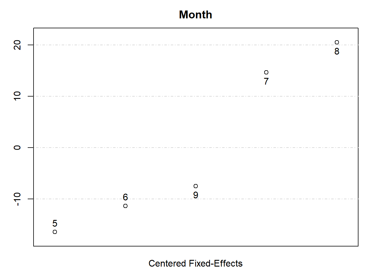
# set up
library(fixest)

# let R know the base dataset (the biggest/ultimate
# dataset that includes everything in your analysis)
base = iris

# rename variables
names(base) = c("y1", "y2", "x1", "x2", "species")

res_multi = feols(
    c(y1, y2) ~ x1 + csw(x2, x2 ^ 2) |
        sw0(species),
    data = base,
    fsplit = ~ species,
    lean = TRUE,
    vcov = "hc1" # can also clustered at the fixed effect level
)
# it's recommended to use vcov at
# estimation stage, not summary stage

summary(res_multi, "compact")
#>         sample   fixef lhs               rhs     (Intercept)                x1
#> 1  Full sample 1        y1 x1 + x2           4.19*** (0.104)  0.542*** (0.076)
#> 2  Full sample 1        y1 x1 + x2 + I(x2^2) 4.27*** (0.101)  0.719*** (0.082)
#> 3  Full sample 1        y2 x1 + x2           3.59*** (0.103) -0.257*** (0.066)
#> 4  Full sample 1        y2 x1 + x2 + I(x2^2) 3.68*** (0.097)    -0.030 (0.078)
#> 5  Full sample species  y1 x1 + x2                            0.906*** (0.076)
#> 6  Full sample species  y1 x1 + x2 + I(x2^2)                  0.900*** (0.077)
#> 7  Full sample species  y2 x1 + x2                              0.155* (0.073)
#> 8  Full sample species  y2 x1 + x2 + I(x2^2)                    0.148. (0.075)
#> 9  setosa      1        y1 x1 + x2           4.25*** (0.474)     0.399 (0.325)
#> 10 setosa      1        y1 x1 + x2 + I(x2^2) 4.00*** (0.504)     0.405 (0.325)
#> 11 setosa      1        y2 x1 + x2           2.89*** (0.416)     0.247 (0.305)
#> 12 setosa      1        y2 x1 + x2 + I(x2^2) 2.82*** (0.423)     0.248 (0.304)
#> 13 setosa      species  y1 x1 + x2                               0.399 (0.325)
#> 14 setosa      species  y1 x1 + x2 + I(x2^2)                     0.405 (0.325)
#> 15 setosa      species  y2 x1 + x2                               0.247 (0.305)
#> 16 setosa      species  y2 x1 + x2 + I(x2^2)                     0.248 (0.304)
#> 17 versicolor  1        y1 x1 + x2           2.38*** (0.423)  0.934*** (0.166)
#> 18 versicolor  1        y1 x1 + x2 + I(x2^2)   0.323 (1.44)   0.901*** (0.164)
#> 19 versicolor  1        y2 x1 + x2           1.25*** (0.275)     0.067 (0.095)
#> 20 versicolor  1        y2 x1 + x2 + I(x2^2)   0.097 (1.01)      0.048 (0.099)
#> 21 versicolor  species  y1 x1 + x2                            0.934*** (0.166)
#> 22 versicolor  species  y1 x1 + x2 + I(x2^2)                  0.901*** (0.164)
#> 23 versicolor  species  y2 x1 + x2                               0.067 (0.095)
#> 24 versicolor  species  y2 x1 + x2 + I(x2^2)                     0.048 (0.099)
#> 25 virginica   1        y1 x1 + x2             1.05. (0.539)  0.995*** (0.090)
#> 26 virginica   1        y1 x1 + x2 + I(x2^2)   -2.39 (2.04)   0.994*** (0.088)
#> 27 virginica   1        y2 x1 + x2             1.06. (0.572)     0.149 (0.107)
#> 28 virginica   1        y2 x1 + x2 + I(x2^2)    1.10 (1.76)      0.149 (0.108)
#> 29 virginica   species  y1 x1 + x2                            0.995*** (0.090)
#> 30 virginica   species  y1 x1 + x2 + I(x2^2)                  0.994*** (0.088)
#> 31 virginica   species  y2 x1 + x2                               0.149 (0.107)
#> 32 virginica   species  y2 x1 + x2 + I(x2^2)                     0.149 (0.108)
#>                  x2          I(x2^2)
#> 1   -0.320. (0.170)
#> 2  -1.52*** (0.307) 0.348*** (0.075)
#> 3    0.364* (0.142)
#> 4  -1.18*** (0.313) 0.446*** (0.074)
#> 5    -0.006 (0.163)
#> 6     0.290 (0.408)   -0.088 (0.117)
#> 7  0.623*** (0.114)
#> 8    0.951* (0.472)   -0.097 (0.125)
#> 9    0.712. (0.418)
#> 10    2.51. (1.47)     -2.91 (2.10)
#> 11    0.702 (0.560)
#> 12     1.27 (2.39)    -0.911 (3.28)
#> 13   0.712. (0.418)
#> 14    2.51. (1.47)     -2.91 (2.10)
#> 15    0.702 (0.560)
#> 16     1.27 (2.39)    -0.911 (3.28)
#> 17   -0.320 (0.364)
#> 18     3.01 (2.31)     -1.24 (0.841)
#> 19 0.929*** (0.244)
#> 20    2.80. (1.65)    -0.695 (0.583)
#> 21   -0.320 (0.364)
#> 22     3.01 (2.31)     -1.24 (0.841)
#> 23 0.929*** (0.244)
#> 24    2.80. (1.65)    -0.695 (0.583)
#> 25    0.007 (0.205)
#> 26    3.50. (2.09)    -0.870 (0.519)
#> 27 0.535*** (0.122)
#> 28    0.503 (1.56)     0.008 (0.388)
#> 29    0.007 (0.205)
#> 30    3.50. (2.09)    -0.870 (0.519)
#> 31 0.535*** (0.122)
#> 32    0.503 (1.56)     0.008 (0.388)

# call the first 3 estimated models only
etable(res_multi[1:3],

       # customize the headers
       headers = c("mod1", "mod2", "mod3"))
#>                   res_multi[1:3].1   res_multi[1:3].2    res_multi[1:3].3
#>                               mod1               mod2                mod3
#> Dependent Var.:                 y1                 y1                  y2
#>
#> Constant         4.191*** (0.1037)  4.266*** (0.1007)   3.587*** (0.1031)
#> x1              0.5418*** (0.0761) 0.7189*** (0.0815) -0.2571*** (0.0664)
#> x2               -0.3196. (0.1700) -1.522*** (0.3072)    0.3640* (0.1419)
#> x2 square                          0.3479*** (0.0748)
#> _______________ __________________ __________________ ___________________
#> S.E. type       Heteroskedas.-rob. Heteroskedas.-rob. Heteroskedast.-rob.
#> Observations                   150                150                 150
#> R2                         0.76626            0.79456             0.21310
#> Adj. R2                    0.76308            0.79034             0.20240
#> ---
#> Signif. codes: 0 '***' 0.001 '**' 0.01 '*' 0.05 '.' 0.1 ' ' 1
12.4.6.2.1 Multiple estimation (Left-hand side)
- When you have multiple interested dependent variables
etable(feols(c(y1, y2) ~ x1 + x2, base))
#>                 feols(c(y1, y2)..1 feols(c(y1, y2) ..2
#> Dependent Var.:                 y1                  y2
#>
#> Constant         4.191*** (0.0970)   3.587*** (0.0937)
#> x1              0.5418*** (0.0693) -0.2571*** (0.0669)
#> x2               -0.3196* (0.1605)    0.3640* (0.1550)
#> _______________ __________________ ___________________
#> S.E. type                      IID                 IID
#> Observations                   150                 150
#> R2                         0.76626             0.21310
#> Adj. R2                    0.76308             0.20240
#> ---
#> Signif. codes: 0 '***' 0.001 '**' 0.01 '*' 0.05 '.' 0.1 ' ' 1
To input a list of dependent variable
depvars <- c("y1", "y2")

res <- lapply(depvars, function(var) {
    res <- feols(xpd(..lhs ~ x1 + x2, ..lhs = var), data = base)
    # summary(res)
})
etable(res)
#>                            model 1             model 2
#> Dependent Var.:                 y1                  y2
#>
#> Constant         4.191*** (0.0970)   3.587*** (0.0937)
#> x1              0.5418*** (0.0693) -0.2571*** (0.0669)
#> x2               -0.3196* (0.1605)    0.3640* (0.1550)
#> _______________ __________________ ___________________
#> S.E. type                      IID                 IID
#> Observations                   150                 150
#> R2                         0.76626             0.21310
#> Adj. R2                    0.76308             0.20240
#> ---
#> Signif. codes: 0 '***' 0.001 '**' 0.01 '*' 0.05 '.' 0.1 ' ' 1
12.4.6.2.2 Multiple estimation (Right-hand side)
Options to write the functions
sw(stepwise): sequentially analyze each elementsy ~ sw(x1, x2)will be estimated asy ~ x1andy ~ x2
sw0(stepwise 0): similar toswbut also estimate a model without the elements in the set firsty ~ sw(x1, x2)will be estimated asy ~ 1andy ~ x1andy ~ x2
csw(cumulative stepwise): sequentially add each element of the set to the formulay ~ csw(x1, x2)will be estimated asy ~ x1andy ~ x1 + x2
csw0(cumulative stepwise 0): similar tocswbut also estimate a model without the elements in the set firsty ~ csw(x1, x2)will be estimated asy~ 1y ~ x1andy ~ x1 + x2
mvsw(multiverse stepwise): all possible combination of the elements in the set (it will get large very quick).mvsw(x1, x2, x3)will besw0(x1, x2, x3, x1 + x2, x1 + x3, x2 + x3, x1 + x2 + x3)
12.4.6.2.3 Split sample estimation
etable(feols(y1 ~ x1 + x2, fsplit = ~ species, data = base))
#>                  feols(y1 ~ x1 +..1 feols(y1 ~ x1 ..2 feols(y1 ~ x1 +..3
#> Sample (species)        Full sample            setosa         versicolor
#> Dependent Var.:                  y1                y1                 y1
#>
#> Constant          4.191*** (0.0970) 4.248*** (0.4114)  2.381*** (0.4493)
#> x1               0.5418*** (0.0693)   0.3990 (0.2958) 0.9342*** (0.1693)
#> x2                -0.3196* (0.1605)   0.7121 (0.4874)   -0.3200 (0.4024)
#> ________________ __________________ _________________ __________________
#> S.E. type                       IID               IID                IID
#> Observations                    150                50                 50
#> R2                          0.76626           0.11173            0.57432
#> Adj. R2                     0.76308           0.07393            0.55620
#>
#>                  feols(y1 ~ x1 +..4
#> Sample (species)          virginica
#> Dependent Var.:                  y1
#>
#> Constant            1.052* (0.5139)
#> x1               0.9946*** (0.0893)
#> x2                  0.0071 (0.1795)
#> ________________ __________________
#> S.E. type                       IID
#> Observations                     50
#> R2                          0.74689
#> Adj. R2                     0.73612
#> ---
#> Signif. codes: 0 '***' 0.001 '**' 0.01 '*' 0.05 '.' 0.1 ' ' 1
12.4.6.2.4 Standard Errors
iid: errors are homoskedastic and independent and identically distributedhetero: errors are heteroskedastic using White correctioncluster: errors are correlated within the cluster groupsnewey_west: (Newey and West 1986) use for time series or panel data. Errors are heteroskedastic and serially correlated.vcov = newey_west ~ id + periodwhereidis the subject id andperiodis time period of the panel.to specify lag period to consider
vcov = newey_west(2) ~ id + periodwhere we’re considering 2 lag periods.
driscoll_kraay(Driscoll and Kraay 1998) use for panel data. Errors are cross-sectionally and serially correlated.vcov = discoll_kraay ~ period
conley: (Conley 1999) for cross-section data. Errors are spatially correlatedvcov = conley ~ latitude + longitudeto specify the distance cutoff,
vcov = vcov_conley(lat = "lat", lon = "long", cutoff = 100, distance = "spherical"), which will use theconley()helper function.
hc: from thesandwichpackagevcov = function(x) sandwich::vcovHC(x, type = "HC1"))
To let R know which SE estimation you want to use, insert vcov = vcov_type ~ variables