18.1 Treatment effect types

This section is based on Paul Testa’s note

Terminology:

• Quantities of causal interest (i.e., treatment effect types)

• Estimands: parameters of interest

• Estimators: procedures to calculate hesitates for the parameters of interest

Sources of bias (according to prof. Luke Keele)

\[ \begin{aligned} &\text{Estimator - True Causal Effect} \\ &= \text{Hidden bias + Misspecification bias + Statistical Noise} \\ &= \text{Due to design + Due to modeling + Due to finite sample} \end{aligned} \]

18.1.1 Average Treatment Effects

Average treatment effect (ATE) is the difference in means of the treated and control groups

Randomization under Experimental Design can provide an unbiased estimate of ATE.

Let \(Y_i(1)\) denote the outcome of individual \(i\) under treatment and

\(Y_i(0)\) denote the outcome of individual \(i\) under control

Then, the treatment effect for individual \(i\) is the difference between her outcome under treatment and control

\[ \tau_i = Y_i(1) - Y_i(0) \]

Without a time machine or dimension portal, we can only observe one of the two event: either individual \(i\) experiences the treatment or she doesn’t.

Then, the ATE as a quantity of interest can come in handy since we can observe across all individuals

\[ ATE = \frac{1}{N} \sum_{i=1}^N \tau_i = \frac{\sum_1^N Y_i(1)}{N} - \frac{\sum_i^N Y_i(0)}{N} \]

With random assignment (i.e., treatment assignment is independent of potential outcome and observables and unobservables), the observed means difference between the two groups is an unbiased estimator of the average treatment effect

\[ E(Y_i (1) |D = 1) = E(Y_i(1)|D=0) = E(Y_i(1)) \\ E(Y_i(0) |D = 1) = E(Y_i(0)|D = 0 ) = E(Y_i(0)) \]

\[ ATE = E(Y_i(1)) - E(Y_i(0)) \]

Alternatively, we can write the potential outcomes model in a regression form

\[ Y_i = Y_i(0) + [Y_i (1) - Y_i(0)] D_i \]

Let \(\beta_{0i} = Y_i (0) ; \beta_{1i} = Y_i(1) - Y_i(0)\), we have

\[ Y_i = \beta_{0i} + \beta_{1i} D_i \]

where

• \(\beta_{0i}\) = outcome if the unit did not receive any treatment

• \(\beta_{1i}\) = treatment effect (i.e., random coefficients for each unit \(i\))

To understand endogeneity (i.e., nonrandom treatment assignment), we can examine a standard linear model

\[ \begin{aligned} Y_i &= \beta_{0i} + \beta_{1i} D_i \\ &= ( \bar{\beta}_{0} + \epsilon_{0i} ) + (\bar{\beta}_{1} + \epsilon_{1i} )D_i \\ &= \bar{\beta}_{0} + \epsilon_{0i} + \bar{\beta}_{1} D_i + \epsilon_{1i} D_i \end{aligned} \]

When you have random assignment, \(E(\epsilon_{0i}) = E(\epsilon_{1i}) = 0\)

• No selection bias: \(D_i \perp e_{0i}\)

• Treatment effect is independent of treatment assignment: \(D_i \perp e_{1i}\)

But otherwise, residuals can correlate with \(D_i\)

For estimation,

• \(\hat{\beta}_1^{OLS}\) is identical to difference in means (i.e., \(Y_i(1) - Y_i(0)\))

• In case of heteroskedasticity (i.e., \(\epsilon_{0i} + D_i \epsilon_{1i} \neq 0\) ), this residual’s variance depends on \(X\) when you have heterogeneous treatment effects (i.e., \(\epsilon_{1i} \neq 0\))

  • Robust SE should still give consistent estimate of \(\hat{\beta}_1\) in this case

  • Alternatively, one can use two-sample t-test on difference in means with unequal variances.

18.1.2 Conditional Average Treatment Effects

Treatment effects can be different for different groups of people. In words, treatment effects can vary across subgroups.

To examine the heterogeneity across groups (e.g., men vs. women), we can estimate the conditional average treatment effects (CATE) for each subgroup

\[ CATE = E(Y_i(1) - Y_i(0) |D_i, X_i)) \]

18.1.3 Intent-to-treat Effects

When we encounter non-compliance (either people suppose to receive treatment don’t receive it, or people suppose to be in the control group receive the treatment), treatment receipt is not independent of potential outcomes and confounders.

In this case, the difference in observed means between the treatment and control groups is not Average Treatment Effects, but Intent-to-treat Effects (ITT). In words, ITT is the treatment effect on those who receive the treatment

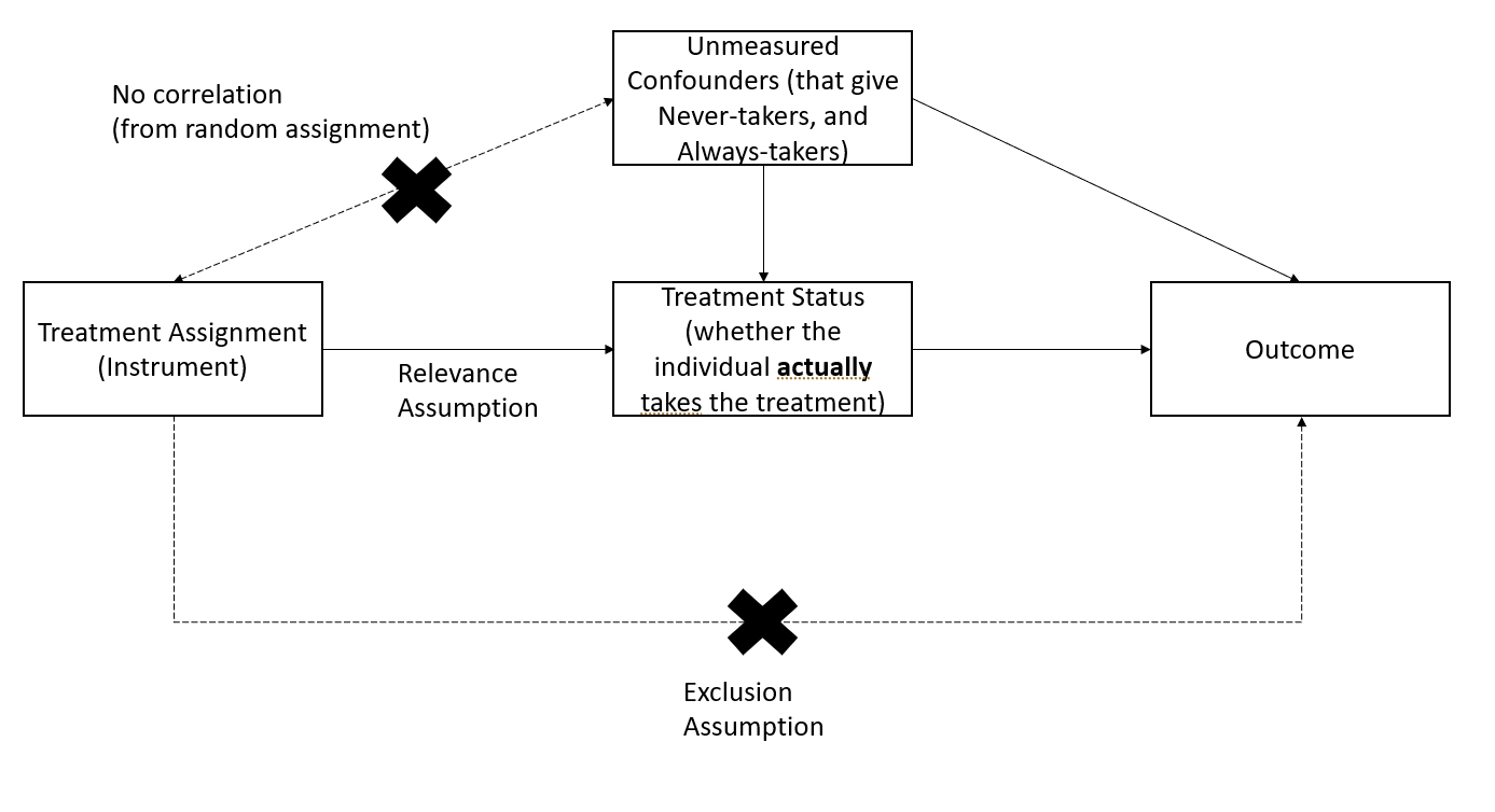
18.1.4 Local Average Treatment Effects

Instead of estimating the treatment effects of those who receive the treatment (i.e., Intent-to-treat Effects), you want to estimate the treatment effect of those who actually comply with the treatment. This is the local average treatment effects (LATE) or complier average causal effects (CACE). I assume we don’t use CATE to denote complier average treatment effect because it was reserved for conditional average treatment effects.

• Using random treatment assignment as an instrument, we can recover the effect of treatment on compliers.

• As the percent of compliers increases, Intent-to-treat Effects and Local Average Treatment Effects converge

• Rule of thumb: SE(LATE) = SE(ITT)/(share of compliers)

• LATE estimate is always greater than the ITT estimate

• LATE can also be estimated using a pure placebo group (Gerber et al. 2010).

• Partial compliance is hard to study, and IV/2SLS estimator is biased, we have to use Bayesian (Long, Little, and Lin 2010; Jin and Rubin 2009, 2008).

18.1.4.1 One-sided noncompliance

• One-sided noncompliance is when in the sample, we only have compliers and never-takers

• With the exclusion restriction (i.e., excludability), never-takers have the same results in the treatment or control group (i.e., never treated)

• With random assignment, we can have the same number of never-takers in the treatment and control groups

• Hence,

\[ LATE = \frac{ITT}{\text{share of compliers}} \]

18.1.4.2 Two-sided noncompliance

• Two-sided noncompliance is when in the sample, we have compliers, never-takers, and always-takers

• To estimate LATE, beyond excludability like in the One-sided noncompliance case, we need to assume that there is no defiers (i.e., monotonicity assumption) (this is excusable in practical studies)

\[ LATE = \frac{ITT}{\text{share of compliers}} \]

18.1.5 Population vs. Sample Average Treatment Effects

See (Imai, King, and Stuart 2008) for when the sample average treatment effect (SATE) diverges from the population average treatment effect (PATE).

To stay consistent, this section uses notations from (Imai, King, and Stuart 2008)’s paper.

In a finite population \(N\), we observe \(n\) observations (\(N>>n\)), where half is in the control and half is in the treatment group.

With unknown data generating process, we have

\[ I_i = \begin{cases} 1 \text{ if unit i is in the sample} \\ 0 \text{ otherwise} \end{cases} \]

\[ T_i = \begin{cases} 1 \text{ if unit i is in the treatment group} \\ 0 \text{ if unit i is in the control group} \end{cases} \]

\[ \text{potential outcome} = \begin{cases} Y_i(1) \text{ if } T_i = 1 \\ Y_i(0) \text{ if } T_i = 0 \end{cases} \]

Observed outcome is

\[ Y_i | I_i = 1= T_i Y_i(1) + (1-T_i)Y_i(0) \]

Since we can never observed both outcome for the same individual, the treatment effect is always unobserved for unit \(i\)

\[ TE_i = Y_i(1) - Y_i(0) \]

Sample average treatment effect is

\[ SATE = \frac{1}{n}\sum_{i \in \{I_i = 1\}} TE_i \]

Population average treatment effect is

\[ PATE = \frac{1}{N}\sum_{i=1}^N TE_i \]

Let \(X_i\) be observables and \(U_i\) be unobservables for unit \(i\)

The baseline estimator for SATE and PATE is

\[ \begin{aligned} D &= \frac{1}{n/2} \sum_{i \in (I_i = 1, T_i = 1)} Y_i - \frac{1}{n/2} \sum_{i \in (I_i = 1 , T_i = 0)} Y_i \\ &= \text{observed sample mean of the treatment group} \\ &- \text{observed sample mean of the control group} \end{aligned} \]

Let \(\Delta\) be the estimation error (deviation from the truth), under an additive model

\[ Y_i(t) = g_t(X_i) + h_t(U_i) \]

The decomposition of the estimation error is

\[ \begin{aligned} PATE - D = \Delta &= \Delta_S + \Delta_T \\ &= (PATE - SATE) + (SATE - D)\\ &= \text{sample selection}+ \text{treatment imbalance} \\ &= (\Delta_{S_X} + \Delta_{S_U}) + (\Delta_{T_X} + \Delta_{T_U}) \\ &= \text{(selection on observed + selection on unobserved)} \\ &+ (\text{treatment imbalance in observed + unobserved}) \end{aligned} \]

18.1.5.1 Estimation Error from Sample Selection

Also known as sample selection error

\[ \Delta_S = PATE - SATE = \frac{N - n}{N}(NATE - SATE) \]

where NATE is the non-sample average treatment effect (i.e., average treatment effect for those in the population but not in your sample:

\[ NATE = \sum_{i\in (I_i = 0)} \frac{TE_i}{N-n} \]

From the equation, to have zero sample selection error (i.e., \(\Delta_S = 0\)), we can either

• Get \(N = n\) by redefining your sample as the population of interest

• \(NATE = SATE\) (e.g., \(TE_i\) is constant over \(i\) in both your selected sample, and those in the population that you did not select)

Note

• When you have heterogeneous treatment effects, random sampling can only warrant sample selection bias, not sample selection error.

• Since we can rarely know the true underlying distributions of the observables (\(X\)) and unobservables (\(U\)), we cannot verify whether the empirical distributions of your observables and unobservables for those in your sample is identical to that of your population (to reduce \(\Delta_S\)). For special case,

  • Say you have census of your population, you can adjust for the observables \(X\) to reduce \(\Delta_{S_X}\), but still you cannot adjust your unobservables (\(U\))

  • Say you are willing to assume \(TE_i\) is constant over

    • \(X_i\), then \(\Delta_{S_X} = 0\)

    • \(U_i\), then \(\Delta_{U}=0\)

18.1.5.2 Estimation Error from Treatment Imbalance

Also known as treatment imbalance error

\[ \Delta_T = SATE - D \]

\(\Delta_T \to 0\) when treatment and control groups are balanced (i.e., identical empirical distributions) for both observables (\(X\)) and unobservables (\(U\))

However, in reality, we can only readjust for observables, not unobservables.

	Blocking	Matching Methods
Definition	Random assignment within strata based on pre-treatment observables	Dropping, repeating or grouping observations to balance covariates between the treatment and control group (Rubin 1973)
Time	Before randomization of treatments	After randomization of treatments
What if the set of covariates used to adjust is irrelevant?	Nothing happens	In the worst case scenario (e.g., these variables are uncorrelated with the treatment assignment, but correlated with the post-treatment variables), matching induces bias that is greater than just using the unadjusted difference in means
Benefits	\(\Delta_{T_X}=0\) (no imbalance on observables). But we don’t know its effect on unobservables imbalance (might reduce if the unobservables are correlated with the observables)	Reduce model dependence, bias, variance, mean-square error

18.1.6 Average Treatment Effects on the Treated and Control

Average Effect of treatment on the Treated (ATT) is

\[ \begin{aligned} ATT &= E(Y_i(1) - Y_i(0)|D_i = 1) \\ &= E(Y_i(1)|D_i = 1) - E(Y_i(0) |D_i = 1) \end{aligned} \]

Average Effect of treatment on the Control (ATC) (i.e., the effect would be for those weren’t treated) is

\[ \begin{aligned} ATC &= E(Y_i(1) - Y_i (0) |D_i =0) \\ &= E(Y_i(1)|D_i = 0) - E(Y_i(0)|D_i = 0) \end{aligned} \]

Under random assignment and full compliance,

\[ ATE = ATT = ATC \]

Sample average treatment effect on the treated is

\[ SATT = \frac{1}{n} \sum_i TE_i \]

where

• \(TE_i\) is the treatment effect for unit \(i\)

• \(n\) is the number of treated units in the sample

• \(i\) belongs the subset (i.e., sample) of the population of interest that is treated.

Population average treatment effect on the treated is

\[ PATT = \frac{1}{N} \sum_i TE_i \]

where

• \(TE_i\) is the treatment effect for unit \(i\)

• \(N\) is the number of treated units in the population

• \(i\) belongs to the population of interest that is treated.

18.1.7 Quantile Average Treatment Effects

Instead of the middle point estimate (ATE), we can also understand the changes in the distribution the outcome variable due to the treatment.

Using quantile regression and more assumptions (Abadie, Angrist, and Imbens 2002; Chernozhukov and Hansen 2005), we can have consistent estimate of quantile treatment effects (QTE), with which we can make inference regarding a given quantile.

18.1.8 Mediation Effects

With additional assumptions (i.e., sequential ignorability (Imai, Keele, and Tingley 2010; Bullock and Ha 2011)), we can examine the mechanism of the treatment on the outcome.

Under the causal framework,

• the indirect effect of treatment via a mediator is called average causal mediation effect (ACME)

• the direct effect of treatment on outcome is the average direct effect (ADE)

More in the Mediation Section 36

18.1.9 Log-odds Treatment Effects

For binary outcome variable, we might be interested in the log-odds of success. See (Freedman 2008) on how to estimate a consistent causal effect.

Alternatively, attributable effects (Rosenbaum 2002) can also be appropriate for binary outcome.