11.2 Solutions to Missing data
11.2.1 Listwise Deletion
Also known as complete case deletion only where you only retain cases with complete data for all features.
Advantages:
Can be applied to any statistical test (SEM, multi-level regression, etc.)
In the case of MCAR, both the parameters estimates and its standard errors are unbiased.
In the case of MAR among independent variables (not depend on the values of dependent variables), then listwise deletion parameter estimates can still be unbiased. (Little 1992) For example, you have a model y=β0+β1X1+β2X2+ϵ if the probability of missing data on X1 is independent of Y, but dependent on the value of X1 and X2, then the model estimates are still unbiased.
- The missing data mechanism the depends on the values of the independent variables are the same as stratified sampling. And stratified sampling does not bias your estimates
- In the case of logistic regression, if the probability of missing data on any variable depends on the value of the dependent variable, but independent of the value of the independent variables, then the listwise deletion will yield biased intercept estimate, but consistent estimates of the slope and their standard errors (Vach and Vach 1994). However, logistic regression will still fail if the probability of missing data is dependent on both the value of the dependent and independent variables.
- Under regression analysis, listwise deletion is more robust than maximum likelihood and multiple imputation when MAR assumption is violated.
Disadvantages:
- It will yield a larger standard errors than other more sophisticated methods discussed later.
- If the data are not MCAR, but MAR, then your listwise deletion can yield biased estimates.
- In other cases than regression analysis, other sophisticated methods can yield better estimates compared to listwise deletion.
11.2.2 Pairwise Deletion
This method could only be used in the case of linear models such as linear regression, factor analysis, or SEM. The premise of this method based on that the coefficient estimates are calculated based on the means, standard deviations, and correlation matrix. Compared to listwise deletion, we still utilized as many correlation between variables as possible to compute the correlation matrix.
Advantages:
If the true missing data mechanism is MCAR, pair wise deletion will yield consistent estimates, and unbiased in large samples
Compared to listwise deletion: (Glasser 1964)
- If the correlation among variables are low, pairwise deletion is more efficient estimates than listwise
- If the correlations among variables are high, listwise deletion is more efficient than pairwise.
Disadvantages:
- If the data mechanism is MAR, pairwise deletion will yield biased estimates.
- In small sample, sometimes covariance matrix might not be positive definite, which means coefficients estimates cannot be calculated.
Note: You need to read carefully on how your software specify the sample size because it will alter the standard errors.
11.2.3 Dummy Variable Adjustment
Also known as Missing Indicator Method or Proxy Variable
Add another variable in the database to indicate whether a value is missing.
Create 2 variables
D={1data on X are missing0otherwise
X∗={Xdata are availablecdata are missing
Note: A typical choice for c is usually the mean of X
Interpretation:
- Coefficient of D is the the difference in the expected value of Y between the group with data and the group without data on X.
- Coefficient of X∗ is the effect of the group with data on Y
Disadvantages:
- This method yields biased estimates of the coefficient even in the case of MCAR (Jones 1996)
11.2.4 Imputation
11.2.4.1 Mean, Mode, Median Imputation
Bad:
- Mean imputation does not preserve the relationships among variables
- Mean imputation leads to An Underestimate of Standard Errors → you’re making Type I errors without realizing it.
- Biased estimates of variances and covariances (Haitovsky 1968)
- In high-dimensions, mean substitution cannot account for dependence structure among features.
11.2.4.2 Maximum Likelihood
When missing data are MAR and monotonic (such as in the case of panel studies), ML can be adequately in estimating coefficients.
Monotonic means that if you are missing data on X1, then that observation also has missing data on all other variables that come after it.
ML can generally handle linear models, log-linear model, but beyond that, ML still lacks both theory and software to implement.
11.2.4.2.1 Expectation-Maximization Algorithm (EM Algorithm)
An iterative process:
- Other variables are used to impute a value (Expectation).
- Check whether the value is most likely (Maximization).
- If not, it re-imputes a more likely value.
You start your regression with your estimates based on either listwise deletion or pairwise deletion. After regressing missing variables on available variables, you obtain a regression model. Plug the missing data back into the original model, with modified variances and covariances For example, if you have missing data on Xij you would regress it on available data of Xi(j), then plug the expected value of Xij back with its X2ij turn into X2ij+s2j(j) where s2j(j) stands for the residual variance from regressing Xij on Xi(j) With the new estimated model, you rerun the process until the estimates converge.
Advantages:
- Easy to use
- Preserves the relationship with other variables (important if you use Factor Analysis or Linear Regression later on), but best in the case of Factor Analysis, which doesn’t require standard error of individuals item.
Disadvantages:
- Standard errors of the coefficients are incorrect (biased usually downward - underestimate)
- Models with overidentification, the estimates will not be efficient
11.2.4.3 Multiple Imputation
MI is designed to use “the Bayesian model-based approach to create procedures, and the frequentist (randomization-based approach) to evaluate procedures”. (Rubin 1996)
MI estimates have the same properties as ML when the data is MAR
- Consistent
- Asymptotically efficient
- Asymptotically normal
MI can be applied to any type of model, unlike Maximum Likelihood that is only limited to a small set of models.
A drawback of MI is that it will produce slightly different estimates every time you run it. To avoid such problem, you can set seed when doing your analysis to ensure its reproducibility.
11.2.4.3.1 Single Random Imputation
Random draws form the residual distribution of each imputed variable and add those random numbers to the imputed values.
For example, if we have missing data on X, and it’s MCAR, then
Regress X on Y (Listwise Deletion method) to get its residual distribution.
For every missing value on X, we substitute with ~xi=^xi+ρui where
- ui is a random draw from a standard normal distribution
- xi is the predicted value from the regression of X and Y
- ρ is the standard deviation of the residual distribution of X regressed on Y.
However, the model you run with the imputed data still thinks that your data are collected, not imputed, which leads your standard error estimates to be too low and test statistics too high.
To address this problem, we need to repeat the imputation process which leads us to repeated imputation or multiple random imputation.
11.2.4.3.2 Repeated Imputation
“Repeated imputations are draws from the posterior predictive distribution of the missing values under a specific model , a particular Bayesian model for both the data and the missing mechanism”.(Rubin 1996)
Repeated imputation, also known as, multiple random imputation, allows us to have multiple “completed” data sets. The variability across imputations will adjust the standard errors upward.
The estimate of the standard error of ˉr (mean correlation estimates between X and Y) is SE(ˉr)=√1M∑ks2k+(1+1M)(1M−1)∑k(rk−ˉr)2 where M is the number of replications, rk is the the correlation in replication k, sk is the estimated standard error in replication k.
However, this method still considers the parameter in predicting ˜x is still fixed, which means we assume that we are using the true parameters to predict ˜x. To overcome this challenge, we need to introduce variability into our model for ˜x by treating the parameters as a random variables and use Bayesian posterior distribution of the parameters to predict the parameters.
However, if your sample is large and the proportion of missing data is small, the extra Bayesian step might not be necessary. If your sample is small or the proportion of missing data is large, the extra Bayesian step is necessary.
Two algorithms to get random draws of the regression parameters from its posterior distribution:
- Data Augmentation
- Sampling importance/resampling (SIR)
Authors have argued for SIR superiority due to its computer time (G. King et al. 2001)
11.2.4.3.2.1 Data Augmentation
Steps for data augmentation:
- Choose starting values for the parameters (e.g., for multivariate normal, choose means and covariance matrix). These values can come from previous values, expert knowledge, or from listwise deletion or pairwise deletion or EM estimation.
- Based on the current values of means and covariances calculate the coefficients estimates for the equation that variable with missing data is regressed on all other variables (or variables that you think will help predict the missing values, could also be variables that are not in the final estimation model)
- Use the estimates in step (2) to predict values for missing values. For each predicted value, add a random error from the residual normal distribution for that variable.
- From the “complete” data set, recalculate the means and covariance matrix. And take a random draw from the posterior distribution of the means and covariances with Jeffreys’ prior.
- Using the random draw from step (4), repeat step (2) to (4) until the means and covariances stabilize (converged).
The iterative process allows us to get random draws from the joint posterior distribution of both data nd parameters, given the observed data.
Rules of thumb regarding convergence:
- The higher the proportion of missing, the more iterations
- the rate of convergence for EM algorithm should be the minimum threshold for DA.
- You can also check if your distribution has been converged by diagnostic statistics Can check Bayesian Diagnostics for some introduction.
Types of chains
Parallel: Run a separate chain of iterations for each of data set. Different starting values are encouraged. For example, one could use bootstrap to generate different data set with replacement, and for each data set, calculate the starting values by EM estimates.
- Pro: Run faster, and less likely to have dependence in the resulting data sets.
- Con: Sometimes it will not converge
Sequential one long chain of data augmentation cycles. After burn-in and thinning, you will have to data sets
- Pro: Converged to the true posterior distribution is more likely.
- Con: The resulting data sets are likely to be dependent. Remedies can be thinning and burn-in.
Note on Non-normal or categorical data The normal-based methods still work well, but you will need to do some transformation. For example,
- If the data is skewed, then log-transform, then impute the exponentiate to have the missing data back to its original metric.
- If the data is proportion, logit-transform, impute, then de-transform the missing data.
If you want to impute non-linear relationship, such as interaction between 2 variables and 1 variable is categorical. You can do separate imputation for different levels of that variable separately, then combined for the final analysis.
- If all variables that have missing data are categorical, then unrestricted multinomial model or log-linear model is recommended.
- If a single categorical variable, logistic (logit) regression would be sufficient.
11.2.4.4 Nonparametric/ Semiparametric Methods
11.2.4.4.1 Hot Deck Imputation
- Used by U.S. Census Bureau for public datasets
- approximate Bayesian bootstrap
- A randomly chosen value from an individual in the sample who has similar values on other variables. In other words, find all the sample subjects who are similar on other variables, then randomly choose one of their values on the missing variable.
When we have n1 cases with complete data on Y and n0 cases with missing data on Y
- Step 1: From n1, take a random sample (with replacement) of n1 cases
- Step 2: From the retrieved sample take a random sample (with replacement) of n0 cases
- Step 3: Assign the n0 cases in step 2 to n0 missing data cases.
- Step 4: Repeat the process for every variable.
- Step 5: For multiple imputation, repeat the four steps multiple times.
Note:
If we skip step 1, it reduce variability for estimating standard errors.
Good:
- Constrained to only possible values.
- Since the value is picked at random, it adds some variability, which might come in handy when calculating standard errors.
Challenge: how can you define “similar” here.
11.2.4.4.2 Cold Deck Imputation
Contrary to Hot Deck, Cold Deck choose value systematically from an observation that has similar values on other variables, which remove the random variation that we want.
Donor samples of “cold-deck” imputation come from a different data set.
11.2.4.4.3 Predictive Mean Matching
Steps:
- Regress Y on X (matrix of covariates) for the n1 (i.e., non-missing cases) to get coefficients b (a k×1 vector) and residual variance estimates s2
- Draw randomly from the posterior predictive distribution of the residual variance (assuming a noninformative prior) by calculating (n1−k)s2χ2, where χ2 is a random draw from a χ2n1−k and let s2[1] be an i-th random draw
- Randomly draw from the posterior distribution of the coefficients b, by drawing from MVN(b,s2[1](X′X)−1), where X is an n1×k matrix of X values. Then we have b1
- Using step 1, we can calculate standardized residuals for n1 cases: ei=yi−bxi√s2(1−k/n1)
- Randomly draw a sample (with replacement) of n0 from the n1 residuals in step 4
- With n0 cases, we can calculate imputed values of Y: yi=b[1]xi+s[1]ei where ei are taken from step 5, and b[1] taken from step 3, and s[1] taken from step 2.
- Repeat steps 2 through 6 except for step 4.
Notes:
- can be used for multiple variables where each variable is imputed using all other variables as predictor.
- can also be used for heteroskedasticity in imputed values.
Example from Statistics Globe
set.seed(918273) # Seed
N  <- 3000                                    # Sample size
y  <- round(runif(N,-10, 10))                 # Target variable Y
x1 <- y + round(runif(N, 0, 50))              # Auxiliary variable 1
x2 <- round(y + 0.25 * x1 + rnorm(N,-3, 15))  # Auxiliary variable 2
x3 <- round(0.1 * x1 + rpois(N, 2))           # Auxiliary variable 3
# (categorical variable)
x4 <- as.factor(round(0.02 * y + runif(N)))   # Auxiliary variable 4

# Insert 20% missing data in Y
y[rbinom(N, 1, 0.2) == 1] <- NA

data <- data.frame(y, x1, x2, x3, x4)         # Store data in dataset
head(data) # First 6 rows of our data
#>    y x1  x2 x3 x4
#> 1  8 38  -3  6  1
#> 2  1 50  -9  5  0
#> 3  5 43  20  5  1
#> 4 NA  9  13  3  0
#> 5 -4 40 -10  6  0
#> 6 NA 29  -6  5  1

library("mice") # Load mice package

##### Impute data via predictive mean matching (single imputation)#####

imp_single <- mice(data, m = 1, method = "pmm") # Impute missing values
#>
#>  iter imp variable
#>   1   1  y
#>   2   1  y
#>   3   1  y
#>   4   1  y
#>   5   1  y
data_imp_single <- complete(imp_single)         # Store imputed data
# head(data_imp_single)

# Since single imputation underestiamtes stnadard errors,
# we use multiple imputaiton

##### Predictive mean matching (multiple imputation) #####

# Impute missing values multiple times
imp_multi <- mice(data, m = 5, method = "pmm")
#>
#>  iter imp variable
#>   1   1  y
#>   1   2  y
#>   1   3  y
#>   1   4  y
#>   1   5  y
#>   2   1  y
#>   2   2  y
#>   2   3  y
#>   2   4  y
#>   2   5  y
#>   3   1  y
#>   3   2  y
#>   3   3  y
#>   3   4  y
#>   3   5  y
#>   4   1  y
#>   4   2  y
#>   4   3  y
#>   4   4  y
#>   4   5  y
#>   5   1  y
#>   5   2  y
#>   5   3  y
#>   5   4  y
#>   5   5  y
data_imp_multi_all <-
    # Store multiply imputed data
    complete(imp_multi,
             "repeated",
             include = TRUE)

data_imp_multi <-
    # Combine imputed Y and X1-X4 (for convenience)
    data.frame(data_imp_multi_all[, 1:6], data[, 2:5])

head(data_imp_multi)
#>   y.0 y.1 y.2 y.3 y.4 y.5 x1  x2 x3 x4
#> 1   8   8   8   8   8   8 38  -3  6  1
#> 2   1   1   1   1   1   1 50  -9  5  0
#> 3   5   5   5   5   5   5 43  20  5  1
#> 4  NA   1  -2  -4   9  -8  9  13  3  0
#> 5  -4  -4  -4  -4  -4  -4 40 -10  6  0
#> 6  NA   4   7   7   6   0 29  -6  5  1
Example from UCLA Statistical Consulting
library(mice)
library(VIM)
library(lattice)
library(ggplot2)
## set observations to NA
anscombe <- within(anscombe, {
    y1[1:3] <- NA
    y4[3:5] <- NA
})
## view
head(anscombe)
#>   x1 x2 x3 x4   y1   y2    y3   y4
#> 1 10 10 10  8   NA 9.14  7.46 6.58
#> 2  8  8  8  8   NA 8.14  6.77 5.76
#> 3 13 13 13  8   NA 8.74 12.74   NA
#> 4  9  9  9  8 8.81 8.77  7.11   NA
#> 5 11 11 11  8 8.33 9.26  7.81   NA
#> 6 14 14 14  8 9.96 8.10  8.84 7.04

## check missing data patterns
md.pattern(anscombe)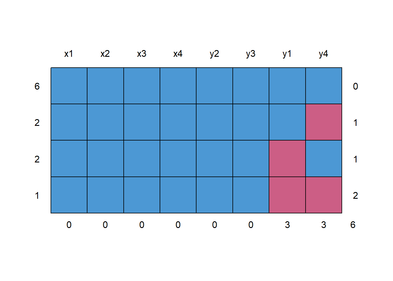
#> x1 x2 x3 x4 y2 y3 y1 y4
#> 6 1 1 1 1 1 1 1 1 0
#> 2 1 1 1 1 1 1 1 0 1
#> 2 1 1 1 1 1 1 0 1 1
#> 1 1 1 1 1 1 1 0 0 2
#> 0 0 0 0 0 0 3 3 6
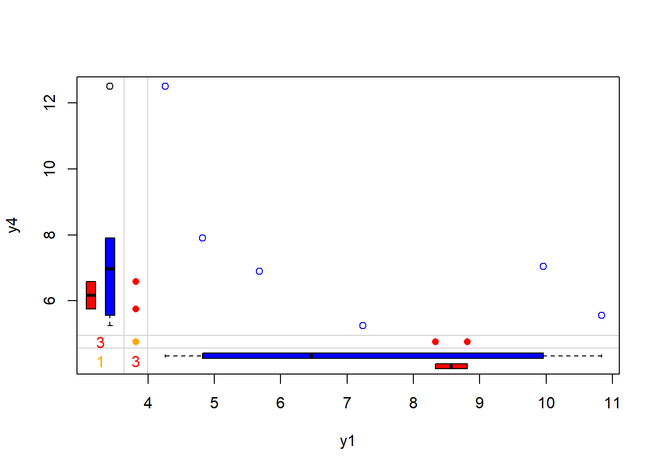
## Number of observations per patterns for all pairs of variables
p <- md.pairs(anscombe)
p
#> $rr
#> x1 x2 x3 x4 y1 y2 y3 y4
#> x1 11 11 11 11 8 11 11 8
#> x2 11 11 11 11 8 11 11 8
#> x3 11 11 11 11 8 11 11 8
#> x4 11 11 11 11 8 11 11 8
#> y1 8 8 8 8 8 8 8 6
#> y2 11 11 11 11 8 11 11 8
#> y3 11 11 11 11 8 11 11 8
#> y4 8 8 8 8 6 8 8 8
#>
#> $rm
#> x1 x2 x3 x4 y1 y2 y3 y4
#> x1 0 0 0 0 3 0 0 3
#> x2 0 0 0 0 3 0 0 3
#> x3 0 0 0 0 3 0 0 3
#> x4 0 0 0 0 3 0 0 3
#> y1 0 0 0 0 0 0 0 2
#> y2 0 0 0 0 3 0 0 3
#> y3 0 0 0 0 3 0 0 3
#> y4 0 0 0 0 2 0 0 0
#>
#> $mr
#> x1 x2 x3 x4 y1 y2 y3 y4
#> x1 0 0 0 0 0 0 0 0
#> x2 0 0 0 0 0 0 0 0
#> x3 0 0 0 0 0 0 0 0
#> x4 0 0 0 0 0 0 0 0
#> y1 3 3 3 3 0 3 3 2
#> y2 0 0 0 0 0 0 0 0
#> y3 0 0 0 0 0 0 0 0
#> y4 3 3 3 3 2 3 3 0
#>
#> $mm
#> x1 x2 x3 x4 y1 y2 y3 y4
#> x1 0 0 0 0 0 0 0 0
#> x2 0 0 0 0 0 0 0 0
#> x3 0 0 0 0 0 0 0 0
#> x4 0 0 0 0 0 0 0 0
#> y1 0 0 0 0 3 0 0 1
#> y2 0 0 0 0 0 0 0 0
#> y3 0 0 0 0 0 0 0 0
#> y4 0 0 0 0 1 0 0 3rr= number of observations where both pairs of values are observedrm= the number of observations where both variables are missing valuesmr= the number of observations where the first variable’s value (e.g. the row variable) is observed and second (or column) variable is missingmm= the number of observations where the second variable’s value (e.g. the col variable) is observed and first (or row) variable is missing
## 5 imputations for all missing values
imp1 <- mice(anscombe, m = 5)
#>
#>  iter imp variable
#>   1   1  y1  y4
#>   1   2  y1  y4
#>   1   3  y1  y4
#>   1   4  y1  y4
#>   1   5  y1  y4
#>   2   1  y1  y4
#>   2   2  y1  y4
#>   2   3  y1  y4
#>   2   4  y1  y4
#>   2   5  y1  y4
#>   3   1  y1  y4
#>   3   2  y1  y4
#>   3   3  y1  y4
#>   3   4  y1  y4
#>   3   5  y1  y4
#>   4   1  y1  y4
#>   4   2  y1  y4
#>   4   3  y1  y4
#>   4   4  y1  y4
#>   4   5  y1  y4
#>   5   1  y1  y4
#>   5   2  y1  y4
#>   5   3  y1  y4
#>   5   4  y1  y4
#>   5   5  y1  y4

## linear regression for each imputed data set - 5 regression are run
fitm <- with(imp1, lm(y1 ~ y4 + x1))
summary(fitm)
#> # A tibble: 15 × 6
#>    term        estimate std.error statistic p.value  nobs
#>    <chr>          <dbl>     <dbl>     <dbl>   <dbl> <int>
#>  1 (Intercept)    8.60      2.67      3.23  0.0121     11
#>  2 y4            -0.533     0.251    -2.12  0.0667     11
#>  3 x1             0.334     0.155     2.16  0.0628     11
#>  4 (Intercept)    4.19      2.93      1.43  0.190      11
#>  5 y4            -0.213     0.273    -0.782 0.457      11
#>  6 x1             0.510     0.167     3.05  0.0159     11
#>  7 (Intercept)    6.51      2.35      2.77  0.0244     11
#>  8 y4            -0.347     0.215    -1.62  0.145      11
#>  9 x1             0.395     0.132     3.00  0.0169     11
#> 10 (Intercept)    5.48      3.02      1.81  0.107      11
#> 11 y4            -0.316     0.282    -1.12  0.295      11
#> 12 x1             0.486     0.173     2.81  0.0230     11
#> 13 (Intercept)    7.12      1.81      3.92  0.00439    11
#> 14 y4            -0.436     0.173    -2.53  0.0355     11
#> 15 x1             0.425     0.102     4.18  0.00308    11

## pool coefficients and standard errors across all 5 regression models
pool(fitm)
#> Class: mipo    m = 5
#>          term m   estimate       ubar           b           t dfcom       df
#> 1 (Intercept) 5  6.3808015 6.72703243 2.785088109 10.06913816     8 3.902859
#> 2          y4 5 -0.3690455 0.05860053 0.014674911  0.07621042     8 4.716160
#> 3          x1 5  0.4301588 0.02191260 0.004980516  0.02788922     8 4.856052
#>         riv    lambda       fmi
#> 1 0.4968172 0.3319158 0.5254832
#> 2 0.3005074 0.2310693 0.4303733
#> 3 0.2727480 0.2142985 0.4143230

## output parameter estimates
summary(pool(fitm))
#>          term   estimate std.error statistic       df    p.value
#> 1 (Intercept)  6.3808015 3.1731905  2.010847 3.902859 0.11643863
#> 2          y4 -0.3690455 0.2760624 -1.336819 4.716160 0.24213491
#> 3          x1  0.4301588 0.1670007  2.575791 4.856052 0.05107581
11.2.4.4.4 Stochastic Imputation
Regression imputation + random residual = Stochastic Imputation
Most multiple imputation is based off of some form of stochastic regression imputation.
Good:
- Has all the advantage of Regression Imputation
- and also has the random components
Bad:
- might lead to implausible values (e.g. negative values)
- can’t handle heteroskadastic data
Note
Multiple Imputation usually based on some form of stochastic regression imputation.
# Income data

set.seed(91919)                              # Set seed
N <- 1000                                    # Sample size

income <- round(rnorm(N, 0, 500))            # Create some synthetic income data
income[income < 0] <- income[income < 0] * (- 1)

x1 <- income + rnorm(N, 1000, 1500)          # Auxiliary variables
x2 <- income + rnorm(N, - 5000, 2000)

income[rbinom(N, 1, 0.1) == 1] <- NA         # Create 10% missingness in income

data_inc_miss <- data.frame(income, x1, x2)
Single stochastic regression imputation
imp_inc_sri  <- mice(data_inc_miss, method = "norm.nob", m = 1)
#>
#>  iter imp variable
#>   1   1  income
#>   2   1  income
#>   3   1  income
#>   4   1  income
#>   5   1  income
data_inc_sri <- complete(imp_inc_sri)
Single predictive mean matching
imp_inc_pmm  <- mice(data_inc_miss, method = "pmm", m = 1)
#>
#>  iter imp variable
#>   1   1  income
#>   2   1  income
#>   3   1  income
#>   4   1  income
#>   5   1  income
data_inc_pmm <- complete(imp_inc_pmm)
Stochastic regression imputation contains negative values
data_inc_sri$income[data_inc_sri$income < 0]
#> [1]  -66.055957  -96.980053  -28.921432   -4.175686  -54.480798  -27.207102
#> [7] -143.603500  -80.960488
# No values below 0
data_inc_pmm$income[data_inc_pmm$income < 0]
#> numeric(0)
Evidence for heteroskadastic data
# Heteroscedastic data

set.seed(654654)                             # Set seed
N <- 1:5000                                  # Sample size

a <- 0
b <- 1
sigma2 <- N^2
eps <- rnorm(N, mean = 0, sd = sqrt(sigma2))

y <- a + b * N + eps                         # Heteroscedastic variable
x <- 30 * N + rnorm(N[length(N)], 1000, 200) # Correlated variable

y[rbinom(N[length(N)], 1, 0.3) == 1] <- NA   # 30% missing

data_het_miss <- data.frame(y, x)
Single stochastic regression imputation
imp_het_sri  <- mice(data_het_miss, method = "norm.nob", m = 1)
#>
#>  iter imp variable
#>   1   1  y
#>   2   1  y
#>   3   1  y
#>   4   1  y
#>   5   1  y
data_het_sri <- complete(imp_het_sri)
Single predictive mean matching
imp_het_pmm <- mice(data_het_miss, method = "pmm", m = 1)
#>
#> iter imp variable
#> 1 1 y
#> 2 1 y
#> 3 1 y
#> 4 1 y
#> 5 1 y
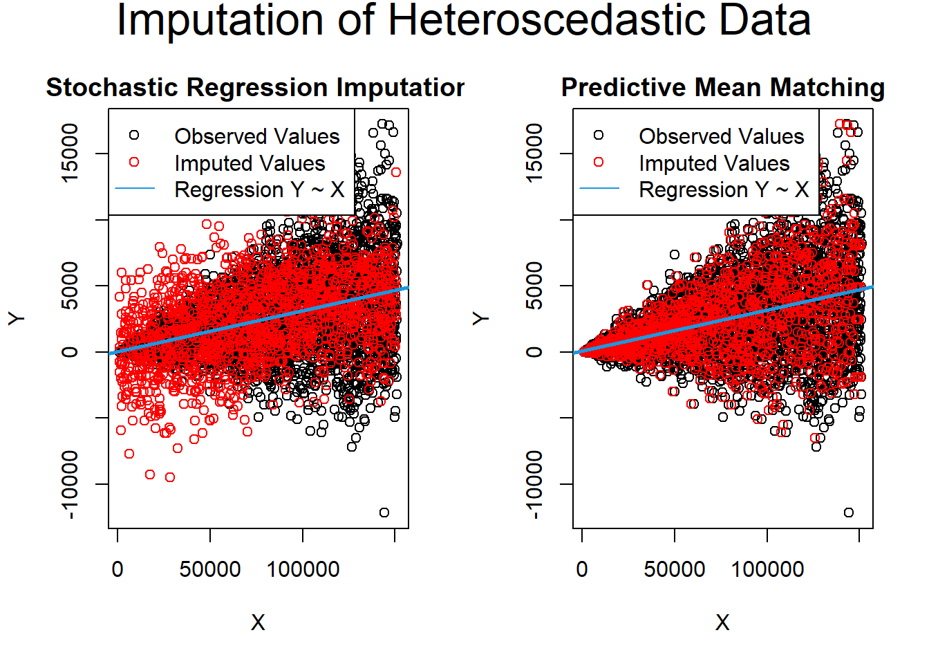
data_het_pmm <- complete(imp_het_pmm)Comparison between predictive mean matching and stochastic regression imputation
par(mfrow = c(1, 2))                              # Both plots in one graphic

# Plot of observed values
plot(x[!is.na(data_het_sri$y)],
     data_het_sri$y[!is.na(data_het_sri$y)],
     main = "",
     xlab = "X",
     ylab = "Y")
# Plot of missing values
points(x[is.na(y)], data_het_sri$y[is.na(y)],
       col = "red")

# Title of plot
title("Stochastic Regression Imputation",
      line = 0.5)

# Regression line
abline(lm(y ~ x, data_het_sri),
       col = "#1b98e0", lwd = 2.5)

# Legend
legend(
  "topleft",
  c("Observed Values", "Imputed Values", "Regression Y ~ X"),
  pch = c(1, 1, NA),
  lty = c(NA, NA, 1),
  col = c("black", "red", "#1b98e0")
)

# Plot of observed values
plot(x[!is.na(data_het_pmm$y)],
     data_het_pmm$y[!is.na(data_het_pmm$y)],
     main = "",
     xlab = "X",
     ylab = "Y")


# Plot of missing values
points(x[is.na(y)], data_het_pmm$y[is.na(y)],
       col = "red")

# Title of plot
title("Predictive Mean Matching",
      line = 0.5)
abline(lm(y ~ x, data_het_pmm),
       col = "#1b98e0", lwd = 2.5)

# Legend
legend(
  "topleft",
  c("Observed Values", "Imputed Values", "Regression Y ~ X"),
  pch = c(1, 1, NA),
  lty = c(NA, NA, 1),
  col = c("black", "red", "#1b98e0")
)

mtext(
  "Imputation of Heteroscedastic Data",
  # Main title of plot
  side = 3,
  line = -1.5,
  outer = TRUE,
  cex = 2
)
11.2.4.5 Regression Imputation
Also known as conditional mean imputation Missing value is based (regress) on other variables.
Good:
Maintain the relationship with other variables (i.e., preserve dependence structure among features, unlike 11.2.4.1).
If the data are MCAR, least-squares coefficients estimates will be consistent, and approximately unbiased in large samples (Gourieroux and Monfort 1981)
- Can have improvement on efficiency by using weighted least squares (Beale and Little 1975) or generalized least squares (Gourieroux and Monfort 1981).
Bad:
- No variability left. treated data as if they were collected.
- Underestimate the standard errors and overestimate test statistics
11.2.4.6 Interpolation and Extrapolation
An estimated value from other observations from the same individual. It usually only works in longitudinal data.
11.2.4.7 K-nearest neighbor (KNN) imputation
The above methods are model-based imputation (regression).
This is an example of neighbor-based imputation (K-nearest neighbor).
For every observation that needs to be imputed, the algorithm identifies ‘k’ closest observations based on some types distance (e.g., Euclidean) and computes the weighted average (weighted based on distance) of these ‘k’ obs.
For a discrete variable, it uses the most frequent value among the k nearest neighbors.
- Distance metrics: Hamming distance.
For a continuous variable, it uses the mean or mode.
Distance metrics:
- Euclidean
- Mahalanobis
- Manhattan
11.2.4.9 Matrix Completion
Impute items missing at random while accounting for dependence between features by using principal components, which is known as matrix completion (James et al. 2013, Sec 12.3)
Consider an n×p feature matrix, X, with element xij, some of which are missing.
Similar to 22.2, we can approximate the matrix X in terms of its leading PCs.
We consider the M principal components that optimize
minA∈Rn×M,B∈Rp×M{∑(i,j)∈O(xij−M∑m=1aimbjm)2}
where O is the set of all observed pairs indices (i,j), a subset of the possible n×p pairs
Once this minimization is solved,
One can impute a missing observation, xij, with ˆxij=∑Mm=1ˆaimˆbjm where ˆaim,ˆbjm are the (i,m) and (j.m) elements, respectively, of the matrices ˆA and ˆB from the minimization, and
One can approximately recover the M principal component scores and loadings, as we did when the data were complete
The challenge here is to solve this minimization problem: the eigen-decomposition non longer applies (as in 22.2
Hence, we have to use iterative algorithm (James et al. 2013 Alg 12.1)
- Create a complete data matrix ˜X of dimension n×p of which the (i,j) element equals
˜xij={xijif (i,j)∈Oˉxjif (i,j)∉O
where ˉxj is the average of the observed values for the jth variable in the incomplete data matrix X
O indexes the observations that are observed in X
- Repeat these 3 steps until some objectives are met
a. Solve
minA∈Rn×M,B∈Rp×M{∑(i,j)∈O(xij−M∑m=1aimbjm)2}
by computing the principal components of ˜X
b. For each element (i,j)∉O, set ˜xij←∑Mm=1ˆaimˆbjm
c. Compute the objective
∑(i,j∈O)(xij−M∑m=1ˆaimˆbjm)2
- Return the estimated missing entries ˜xij,(i,j)∉O