11.6 Application
library(visdat)
library(naniar)
library(ggplot2)
vis_miss()


ggplot(data, aes(x, y)) +
  geom_miss_point() +
  facet_wrap( ~ group)

gg_miss_var(data, facet = group)

gg_miss_upset(data)

gg_miss_fct(x = variable1, fct = variable2)
Read more on The Missing Book by Nicholas Tierney & Allison Horst
How many imputation:
Usually 5. (unless you have extremely high portion of missing, in which case you probably need to check your data again)
According to Rubin, the relative efficiency of an estimate based on \(m\) imputations to infinity imputation is approximately
\[ (1+\frac{\lambda}{m})^{-1} \]
where \(\lambda\) is the rate of missing data
Example 50% of missing data means an estimate based on 5 imputation has standard deviation that is only 5% wider compared to an estimate based on infinity imputation
(\(\sqrt{1+0.5/5}=1.049\))
library(missForest)

#load data
data <- iris

#Generate 10% missing values at Random
set.seed(1)
iris.mis <- prodNA(iris, noNA = 0.1)

#remove categorical variables
iris.mis.cat <- iris.mis
iris.mis <- subset(iris.mis, select = -c(Species))
11.6.1 Imputation with mean / median / mode
# whole data set
e1071::impute(iris.mis, what = "mean")        # replace with mean
e1071::impute(iris.mis, what = "median")      # replace with median

# by variables
Hmisc::impute(iris.mis$Sepal.Length, mean)    # mean
Hmisc::impute(iris.mis$Sepal.Length, median)  # median
Hmisc::impute(iris.mis$Sepal.Length, 0)       # replace specific number
check accuracy
11.6.2 KNN
# library(DMwR2)
# # iris.mis[,!names(iris.mis) %in% c("Sepal.Length")]
# # data should be this line. But since knn cant work with 3 or less variables,
# # we need to use at least 4 variables.
#
# # knn is not appropriate for categorical variables
# knnOutput <-
#   knnImputation(data = iris.mis.cat,
#                 #k = 10,
#                 meth = "median" # could use "median" or "weighAvg")
#                 # should exclude the dependent variable: Sepal.Length
#                 anyNA(knnOutput)
# library(DMwR2)
# actuals <- iris$Sepal.Width[is.na(iris.mis$Sepal.Width)]
# predicteds <- knnOutput[is.na(iris.mis$Sepal.Width), "Sepal.Width"]
# regr.eval(actuals, predicteds)Compared to MAPE (mean absolute percentage error) of mean imputation, we see almost always see improvements.
11.6.3 rpart
For categorical (factor) variables, rpart can handle
library(rpart)
class_mod <-
  rpart(
    Species ~ . - Sepal.Length,
    data = iris.mis.cat[!is.na(iris.mis.cat$Species),],
    method = "class",
    na.action = na.omit
  )  # since Species is a factor, and exclude dependent variable "Sepal.Length"

anova_mod <-
  rpart(
    Sepal.Width ~ . - Sepal.Length,
    data = iris.mis[!is.na(iris.mis$Sepal.Width),],
    method = "anova",
    na.action = na.omit
  )  # since Sepal.Width is numeric.


species_pred <-
  predict(class_mod, iris.mis.cat[is.na(iris.mis.cat$Species),])


width_pred <-
  predict(anova_mod, iris.mis[is.na(iris.mis$Sepal.Width),])
11.6.4 MICE (Multivariate Imputation via Chained Equations)
Assumption: data are MAR
It imputes data per variable by specifying an imputation model for each variable
Example
We have \(X_1, X_2,..,X_k\). If \(X_1\) has missing data, then it is regressed on the rest of the variables. Same procedure applies if \(X_2\) has missing data. Then, predicted values are used in place of missing values.
By default,
- Continuous variables use linear regression.
- Categorical Variables use logistic regression.
Methods in MICE:
- PMM (Predictive Mean Matching) – For numeric variables
logreg(Logistic Regression) – For Binary Variables( with 2 levels)polyreg(Bayesian polytomous regression) – For Factor Variables (>= 2 levels)- Proportional odds model (ordered, >= 2 levels)
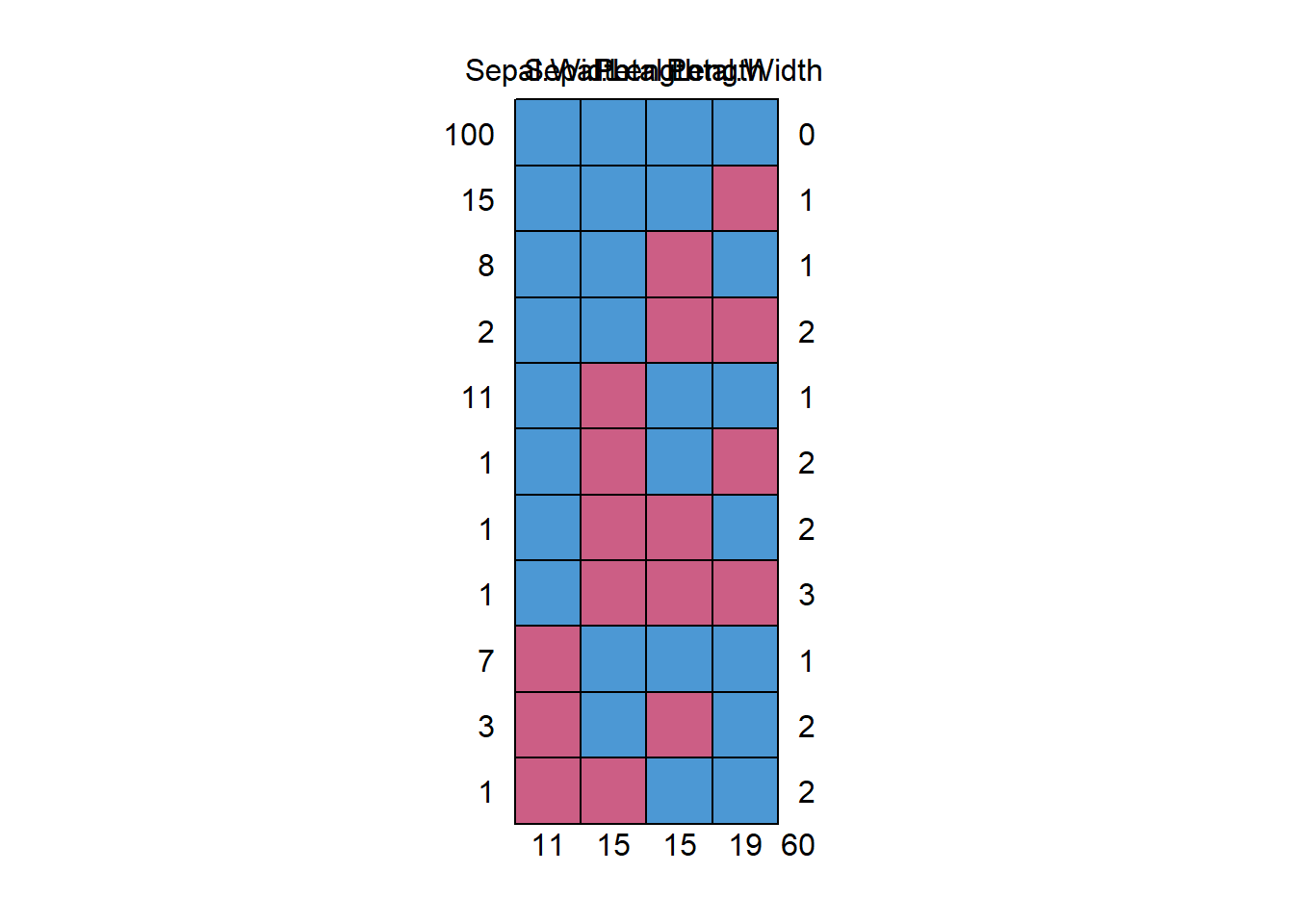
#>     Sepal.Width Sepal.Length Petal.Length Petal.Width
#> 100           1            1            1           1  0
#> 15            1            1            1           0  1
#> 8             1            1            0           1  1
#> 2             1            1            0           0  2
#> 11            1            0            1           1  1
#> 1             1            0            1           0  2
#> 1             1            0            0           1  2
#> 1             1            0            0           0  3
#> 7             0            1            1           1  1
#> 3             0            1            0           1  2
#> 1             0            0            1           1  2
#>              11           15           15          19 60

#plot the missing values
aggr(
  iris.mis,
  col = mdc(1:2),
  numbers = TRUE,
  sortVars = TRUE,
  labels = names(iris.mis),
  cex.axis = .7,
  gap = 3,
  ylab = c("Proportion of missingness", "Missingness Pattern")
)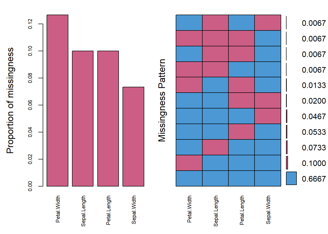
#>
#>  Variables sorted by number of missings:
#>      Variable      Count
#>   Petal.Width 0.12666667
#>  Sepal.Length 0.10000000
#>  Petal.Length 0.10000000
#>   Sepal.Width 0.07333333


mice_plot <- aggr(
  iris.mis,
  col = c('navyblue', 'yellow'),
  numbers = TRUE,
  sortVars = TRUE,
  labels = names(iris.mis),
  cex.axis = .7,
  gap = 3,
  ylab = c("Missing data", "Pattern")
)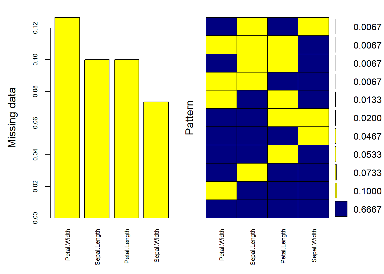
#>
#>  Variables sorted by number of missings:
#>      Variable      Count
#>   Petal.Width 0.12666667
#>  Sepal.Length 0.10000000
#>  Petal.Length 0.10000000
#>   Sepal.Width 0.07333333
Impute Data
imputed_Data <-
    mice(
        iris.mis,
        m = 5, # number of imputed datasets
        maxit = 50, # number of iterations taken to impute missing values
        method = 'pmm', # method used in imputation.
        # Here, we used predictive mean matching


        # other methods can be
        # "pmm": Predictive mean matching
        # "midastouch" : weighted predictive mean matching
        # "sample": Random sample from observed values
        # "cart": classification and regression trees
        # "rf": random forest imputations.
        # "2lonly.pmm": Level-2 class predictive mean matching
        # Other methods based on whether variables are
        # (1) numeric, (2) binary, (3) ordered, (4), unordered
        seed = 500
)summary(imputed_Data)
#> Class: mids
#> Number of multiple imputations: 5
#> Imputation methods:
#> Sepal.Length Sepal.Width Petal.Length Petal.Width
#> "pmm" "pmm" "pmm" "pmm"
#> PredictorMatrix:
#> Sepal.Length Sepal.Width Petal.Length Petal.Width
#> Sepal.Length 0 1 1 1
#> Sepal.Width 1 0 1 1
#> Petal.Length 1 1 0 1
#> Petal.Width 1 1 1 0
#make a density plot
densityplot(imputed_Data)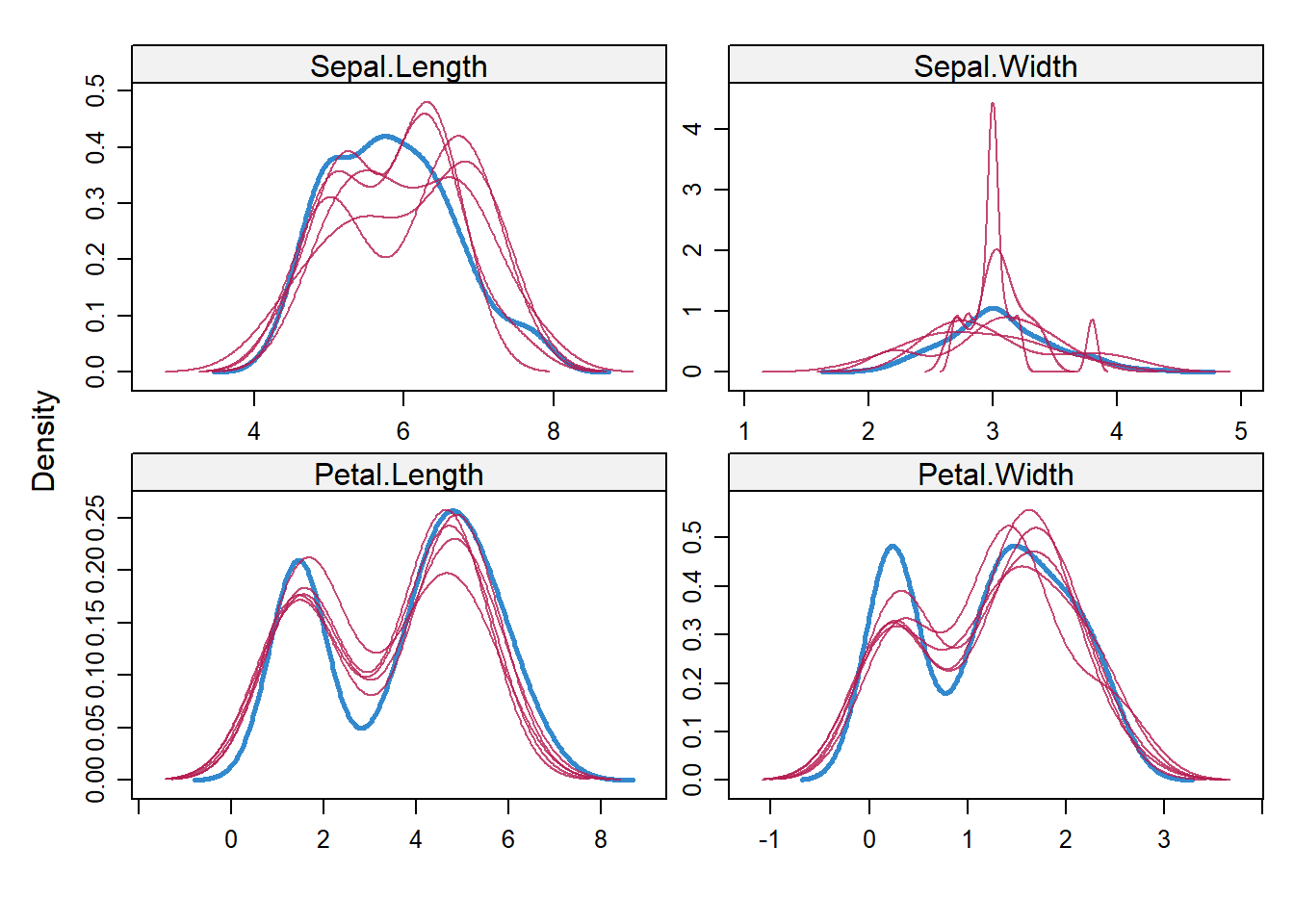
Check imputed dataset
Regression model using imputed datasets
# regression model
fit <-
  with(data = imputed_Data,
       exp = lm(Sepal.Width ~ Sepal.Length + Petal.Width))

#combine results of all 5 models
combine <- pool(fit)
summary(combine)
#>           term   estimate  std.error statistic       df      p.value
#> 1  (Intercept)  1.8963130 0.32453912  5.843095 131.0856 3.838556e-08
#> 2 Sepal.Length  0.2974293 0.06679204  4.453066 130.2103 1.802241e-05
#> 3  Petal.Width -0.4811603 0.07376809 -6.522608 108.8253 2.243032e-09
11.6.5 Amelia
- Use bootstrap based EMB algorithm (faster and robust to impute many variables including cross sectional, time series data etc)
- Use parallel imputation feature using multicore CPUs.
Assumptions
- All variables follow Multivariate Normal Distribution (MVN). Hence, this package works best when data is MVN, or transformation to normality.
- Missing data is Missing at Random (MAR)
Steps:
- m bootstrap samples and applies EMB algorithm to each sample. Then we have m different estimates of mean and variances.
- the first set of estimates are used to impute first set of missing values using regression, then second set of estimates are used for second set and so on.
However, Amelia is different from MICE
- MICE imputes data on variable by variable basis whereas MVN uses a joint modeling approach based on multivariate normal distribution.
- MICE can handle different types of variables while the variables in MVN need to be normally distributed or transformed to approximate normality.
- MICE can manage imputation of variables defined on a subset of data whereas MVN cannot.
- idvars – keep all ID variables and other variables which you don’t want to impute
- noms – keep nominal variables here
#specify columns and run amelia
amelia_fit <-
  amelia(iris.mis,
         m = 5,
         parallel = "multicore",
         noms = "Species")
#> -- Imputation 1 --
#>
#>   1  2  3  4  5  6  7  8
#>
#> -- Imputation 2 --
#>
#>   1  2  3  4  5  6  7  8
#>
#> -- Imputation 3 --
#>
#>   1  2  3  4  5
#>
#> -- Imputation 4 --
#>
#>   1  2  3  4  5  6  7
#>
#> -- Imputation 5 --
#>
#>   1  2  3  4  5  6  7

# access imputed outputs
# amelia_fit$imputations[[1]]
11.6.6 missForest
- an implementation of random forest algorithm (a non parametric imputation method applicable to various variable types). Hence, no assumption about function form of f. Instead, it tries to estimate f such that it can be as close to the data points as possible.
- builds a random forest model for each variable. Then it uses the model to predict missing values in the variable with the help of observed values.
- It yields out of bag imputation error estimate. Moreover, it provides high level of control on imputation process.
- Since bagging works well on categorical variable too, we don’t need to remove them here.
library(missForest)
#impute missing values, using all parameters as default values
iris.imp <- missForest(iris.mis)
# check imputed values
# iris.imp$ximp- check imputation error
- NRMSE is normalized mean squared error. It is used to represent error derived from imputing continuous values.
- PFC (proportion of falsely classified) is used to represent error derived from imputing categorical values.
iris.imp$OOBerror
#>      NRMSE        PFC
#> 0.13631893 0.04477612

#comparing actual data accuracy
iris.err <- mixError(iris.imp$ximp, iris.mis, iris)
iris.err
#>     NRMSE       PFC
#> 0.1501524 0.0625000
This means categorical variables are imputed with 5% error and continuous variables are imputed with 14% error.
This can be improved by tuning the values of mtry and ntree parameter.
mtryrefers to the number of variables being randomly sampled at each split.ntreerefers to number of trees to grow in the forest.
11.6.7 Hmisc
impute()function imputes missing value using user defined statistical method (mean, max, mean). It’s default is median.
aregImpute()allows mean imputation using additive regression, bootstrapping, and predictive mean matching.
- In bootstrapping, different bootstrap resamples are used for each of multiple imputations. Then, a flexible additive model (non parametric regression method) is fitted on samples taken with replacements from original data and missing values (acts as dependent variable) are predicted using non-missing values (independent variable).
- it uses predictive mean matching (default) to impute missing values. Predictive mean matching works well for continuous and categorical (binary & multi-level) without the need for computing residuals and maximum likelihood fit.
Note
- For predicting categorical variables, Fisher’s optimum scoring method is used.
Hmiscautomatically recognizes the variables types and uses bootstrap sample and predictive mean matching to impute missing values.missForestcan outperformHmiscif the observed variables have sufficient information.
Assumption
- linearity in the variables being predicted.
library(Hmisc)
# impute with mean value
iris.mis$imputed_age <- with(iris.mis, impute(Sepal.Length, mean))

# impute with random value
iris.mis$imputed_age2 <-
  with(iris.mis, impute(Sepal.Length, 'random'))

# could also use min, max, median to impute missing value

# using argImpute
impute_arg <-
  # argImpute() automatically identifies the variable type
  # and treats them accordingly.
  aregImpute(
    ~ Sepal.Length + Sepal.Width + Petal.Length + Petal.Width +
      Species,
    data = iris.mis,
    n.impute = 5
  )
#> Iteration 1
Iteration 2
Iteration 3
Iteration 4
Iteration 5
Iteration 6
Iteration 7
Iteration 8

impute_arg # R-squares are for predicted missing values.
#>
#> Multiple Imputation using Bootstrap and PMM
#>
#> aregImpute(formula = ~Sepal.Length + Sepal.Width + Petal.Length +
#>     Petal.Width + Species, data = iris.mis, n.impute = 5)
#>
#> n: 150   p: 5    Imputations: 5      nk: 3
#>
#> Number of NAs:
#> Sepal.Length  Sepal.Width Petal.Length  Petal.Width      Species
#>           11           11           13           24           16
#>
#>              type d.f.
#> Sepal.Length    s    2
#> Sepal.Width     s    2
#> Petal.Length    s    2
#> Petal.Width     s    2
#> Species         c    2
#>
#> Transformation of Target Variables Forced to be Linear
#>
#> R-squares for Predicting Non-Missing Values for Each Variable
#> Using Last Imputations of Predictors
#> Sepal.Length  Sepal.Width Petal.Length  Petal.Width      Species
#>        0.907        0.660        0.978        0.963        0.993

# check imputed variable Sepal.Length
impute_arg$imputed$Sepal.Length
#>     [,1] [,2] [,3] [,4] [,5]
#> 19   5.2  5.2  5.2  5.8  5.7
#> 21   5.1  5.0  5.1  5.7  5.4
#> 31   4.8  5.0  5.2  5.0  4.8
#> 35   4.6  4.9  4.9  4.9  4.8
#> 49   5.0  5.1  5.1  5.1  5.1
#> 62   6.2  5.7  6.0  6.4  5.6
#> 65   5.5  5.5  5.2  5.8  5.5
#> 67   6.5  5.8  5.8  6.3  6.5
#> 82   5.2  5.1  5.7  5.8  5.5
#> 113  6.4  6.5  7.4  7.2  6.3
#> 122  6.2  5.8  5.5  5.8  6.7
11.6.8 mi
- allows graphical diagnostics of imputation models and convergence of imputation process.
- uses Bayesian version of regression models to handle issue of separation.
- automatically detects irregularities in data (e.g., high collinearity among variables).
- adds noise to imputation process to solve the problem of additive constraints.