37.4 Publication Bias
Publication bias occurs when the results of studies influence the likelihood of their being published. Typically, studies with significant, positive, or sensational results are more likely to be published than those with non-significant or negative results. This can skew the perceived effectiveness or results when researchers conduct meta-analyses or literature reviews, leading them to draw inaccurate conclusions.
Example: Imagine pharmaceutical research. If 10 studies are done on a new drug, and only 2 show a positive effect while 8 show no effect, but only the 2 positive studies get published, a later review of the literature might erroneously conclude the drug is effective.
Relation to Other Biases:
Selection Bias: Publication bias is a form of selection bias, where the selection (publication in this case) isn’t random but based on the results of the study.
Confirmation Bias: Like survivorship bias, publication bias can reinforce confirmation bias. Researchers might only find and cite studies that confirm their beliefs, overlooking the unpublished studies that might contradict them.
Let’s simulate an experiment on a new treatment. We’ll assume that the treatment has no effect, but due to random variation, some studies will show significant positive or negative effects.
set.seed(42)

# Number of studies
n <- 100

# Assuming no real effect (effect size = 0)
true_effect <- 0

# Random variation in results
results <- rnorm(n, mean = true_effect, sd = 1)

# Only "significant" results get published
# (arbitrarily defining significant as abs(effect) > 1.5)
published_results <- results[abs(results) > 1.5]

# Average effect for all studies vs. published studies
true_avg_effect <- mean(results)
published_avg_effect <- mean(published_results)

true_avg_effect
#> [1] 0.03251482
published_avg_effect
#> [1] -0.3819601
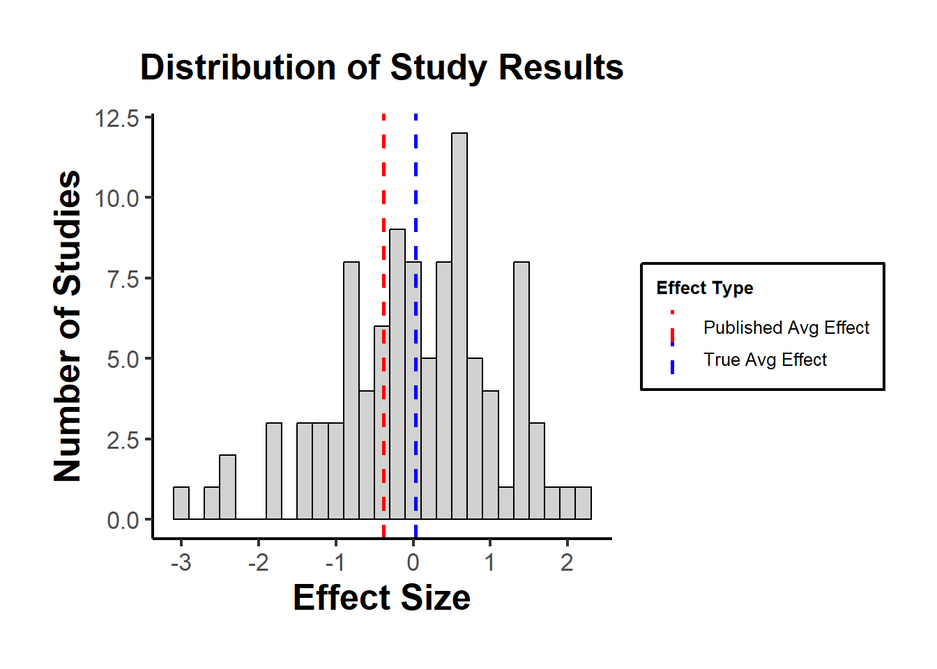
Using a histogram to visualize the distribution of study results, highlighting the “published” studies.
library(ggplot2)

df <- data.frame(results)

p <- ggplot(df, aes(x = results)) +
  geom_histogram(
    binwidth = 0.2,
    fill = "grey",
    color = "black",
    alpha = 0.7
  ) +
  geom_vline(
    aes(xintercept = true_avg_effect,
        color = "True Avg Effect"),
    linetype = "dashed",
    size = 1
  ) +
  geom_vline(
    aes(xintercept = published_avg_effect,
        color = "Published Avg Effect"),
    linetype = "dashed",
    size = 1
  ) +
  scale_color_manual(
    values = c(
      "True Avg Effect" = "blue",
      "Published Avg Effect" = "red"
    ),
    name = "Effect Type"
  ) +
  labs(title = "Distribution of Study Results",
       x = "Effect Size",
       y = "Number of Studies") +
  causalverse::ama_theme()

print(p)
The plot might show that the “True Avg Effect” is around zero, while the “Published Avg Effect” is likely higher or lower, depending on which studies happen to have significant results in the simulation.
Remedies:
Awareness: Understand and accept that publication bias exists, especially when conducting literature reviews or meta-analyses.
Study Registries: Encourage the use of study registries where researchers register their studies before they start. This way, one can see all initiated studies, not just the published ones.
Publish All Results: Journals and researchers should make an effort to publish negative or null results. Some journals, known as “null result journals”, specialize in this.
Funnel Plots and Egger’s Test: In meta-analyses, these are methods to visually and statistically detect publication bias.
Use of Preprints: Promote the use of preprint servers where researchers can upload studies before they’re peer-reviewed, ensuring that results are available regardless of eventual publication status.
p-curve analysis: addresses publication bias and p-hacking by analyzing the distribution of p-values below 0.05 in research studies. It posits that a right-skewed distribution of these p-values indicates a true effect, whereas a left-skewed distribution suggests p-hacking and no true underlying effect. The method includes a “half-curve” test to counteract extensive p-hacking Simonsohn, Simmons, and Nelson (2015).