34.1 Autocorrelation

Assess autocorrelation from residual

# simple regression on time 
simple_ts <- lm(outcome ~ time, data = df)

plot(resid(simple_ts))

# alternatively
acf(resid(simple_ts))

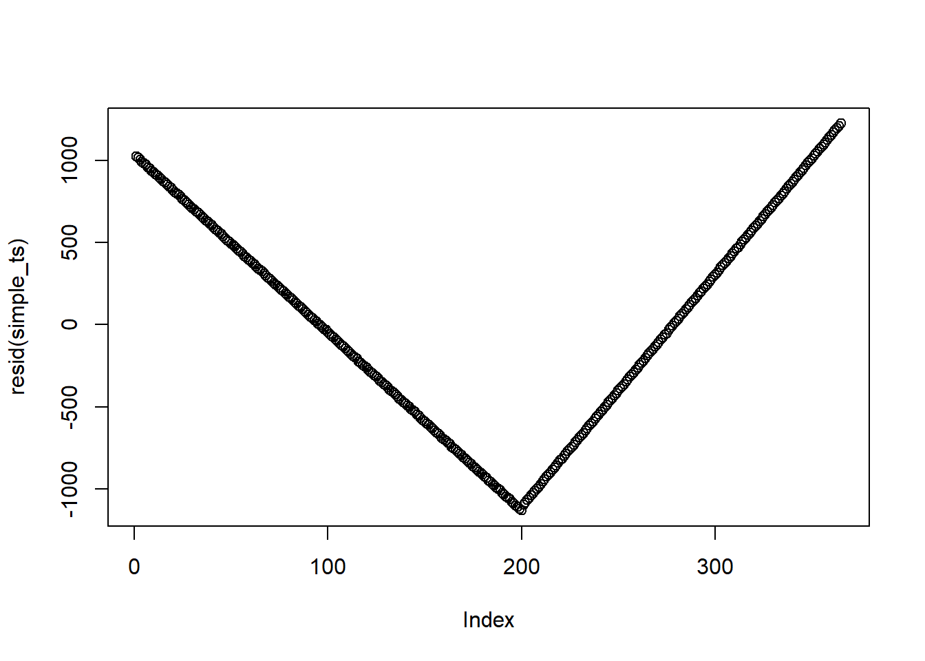
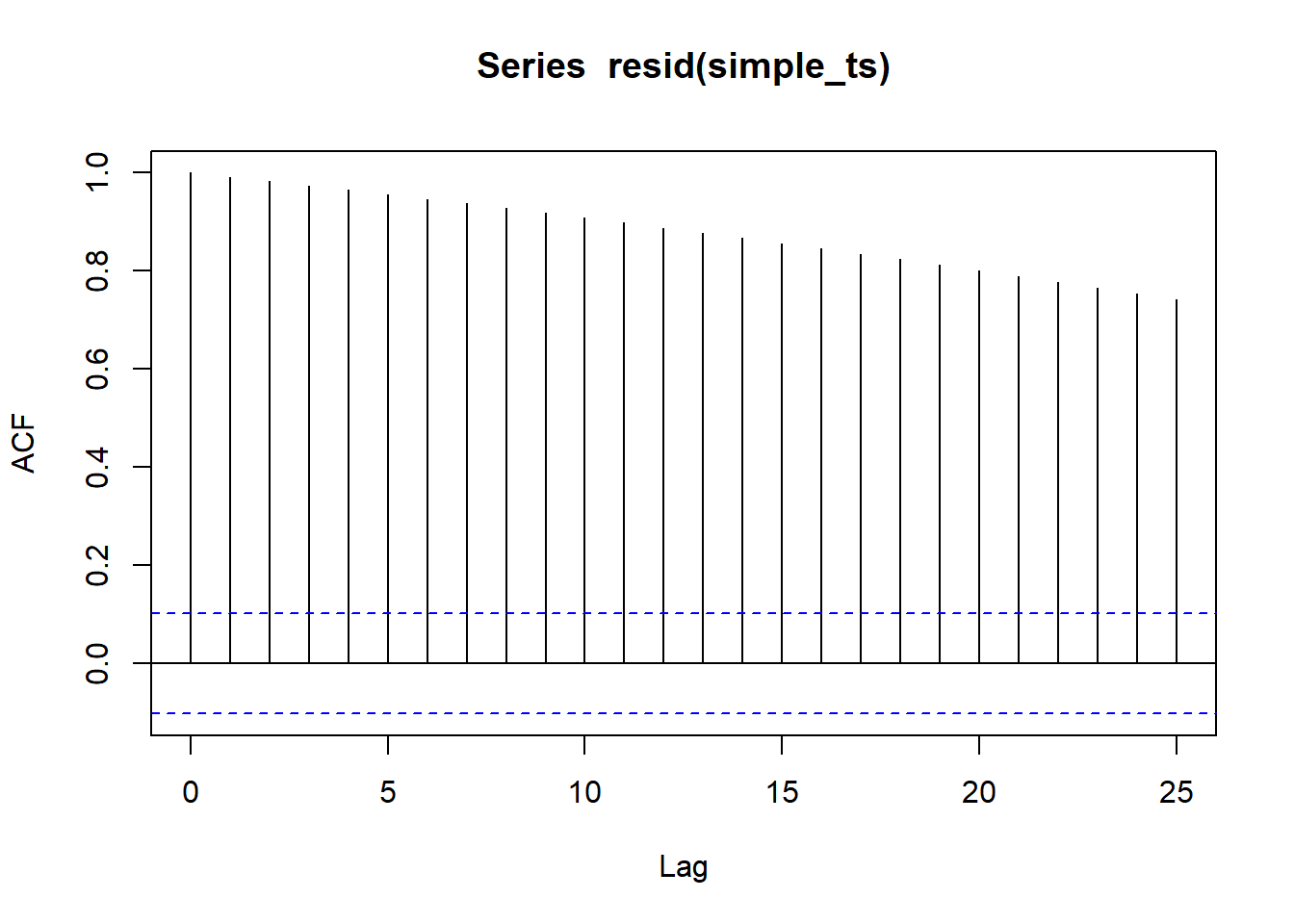
This is not the best example since I created this dataset. But when residuals do have autocorrelation, you should not see any patterns (i.e., points should be randomly distributed on the plot)

To formally test for autocorrelation, we can use the Durbin-Watson test

lmtest::dwtest(df$outcome ~ df$time)
#> 
#>  Durbin-Watson test
#> 
#> data:  df$outcome ~ df$time
#> DW = 0.00037654, p-value < 2.2e-16
#> alternative hypothesis: true autocorrelation is greater than 0

From the p-value, we know that there is autocorrelation in the time series

A solution to this problem is to use more advanced time series analysis (e.g., ARIMA - coming up in the book) to adjust for seasonality and other dependency.

forecast::auto.arima(df$outcome, xreg = as.matrix(df[,-1]))
#> Series: df$outcome 
#> Regression with ARIMA(0,0,0) errors 
#> 
#> Coefficients:
#>       intercept     time  treatment  timesincetreat
#>          9.9042  15.0004    20.0681         25.0001
#> s.e.     0.1513   0.0013     0.2243          0.0022
#> 
#> sigma^2 = 1.148:  log likelihood = -541.12
#> AIC=1092.23   AICc=1092.4   BIC=1111.73