24.5 Sampling distribution
Since the difference between the population means is unknown (that’s why the study was done), the difference is estimated using the sample means. For the reaction time data, we will use subscripts such as \(P\) for phone-users group, and \(C\) for the control group. Then the difference between the two sample means (the statistic) is \(\bar{x}_P - \bar{x}_C\).
The parameter is \(\mu_P - \mu_C\), the difference between the two population means (using a phone, minus not using a phone).
The differences could be compute in the opposite direction (\(\bar{x}_C - \bar{x}_P\)). However, for the reaction-time data, computing differences as the reaction time for phone users, minus the reaction time for non-phone users (controls) probably makes more sense: the differences then refer to how much greater (on average) the reaction times are when students are using phones,
Making clear how the differences are computed is important! Therefore, carefully defining the parameter is important.
The differences could be computed as:
- the reaction time for phone users, minus the reaction time for non-phone users (how much slower the phone users are, on average); or
- the reaction time for non-phone users, minus the reaction time for phone users (how much slower the non-phone users are, on average).
Each sample of students will comprise different students, and will give different reaction times while driving. The means for each group will differ from sample to sample, and the difference between the means will be different for each sample. The difference between the sample means varies from sample to sample, and so has a sampling distribution and standard error.
Definition 24.1 (Sampling distribution of the difference between two sample means) The sampling distribution of the difference between two sample means is described by:
- an approximate normal distribution;
- centred around \(\mu_A - \mu_B\) (the differences between the means);
- with a standard deviation of \(\displaystyle\text{s.e.}( \bar{x}_A - \bar{x}_B)\),
when the appropriate conditions are met.
We don’t give a formula for finding the standard error \(\displaystyle\text{s.e.}( \bar{x}_A - \bar{x}_B)\), so the value of this standard error will be given.For the reaction-time data, the differences between the sample means will have:
- an approximate normal distribution;
- centred around \(\mu_P - \mu_C\) (the differences between the means in the two populations);
- with a standard deviation, called the standard error of the difference, of \(\text{s.e.}(\bar{x}_P - \bar{x}_C) = 19.61\).
We can draw this sampling distribution (Fig. 24.4).
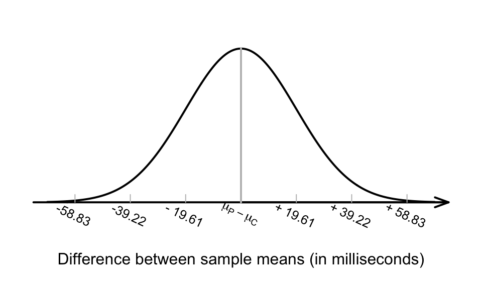
FIGURE 24.4: The sampling distribution of the difference between the reaction times in the phone and control groups (phone, minus control)