35.3 Regression using software

In the population, the intercept is denoted by \(\beta_0\) and the slope is denoted by \(\beta_1\). These population values are unknown, and are estimated by the statistics \(b_0\) and \(b_1\) respectively.
The formulas for computing \(b_0\) and \(b_1\) are ugly, so we will use software to do the calculations. As usual, the values of these population parameters are unknown, and the values of the sample statistics will change from sample to sample (so they have sampling variation).
For the red deer data again
(Fig 33.2),
part of the relevant output is
shown in
Fig. 35.3 (using jamovi) and
Fig. 35.4 (using SPSS).
From the output,
the slope \(b_1\) in the sample is \(b_1=-0.181\),
and the \(y\)-intercept \(b_0\) in the sample is \(b_0 = 4.398\).
That is,
the values of \(b_0\) and \(b_1\) are in the column labelled Estimate in jamovi,
or the column labelled B in SPSS.
These are the values of the two regression coefficients;
then
\[ \hat{y} = 4.398 + (-0.181\times x), \] which is usually written more simply as
\[ \hat{y} = 4.398 - 0.181 x. \]
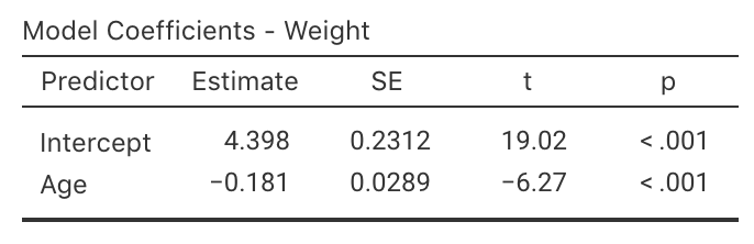
FIGURE 35.3: jamovi output for the red-deer data
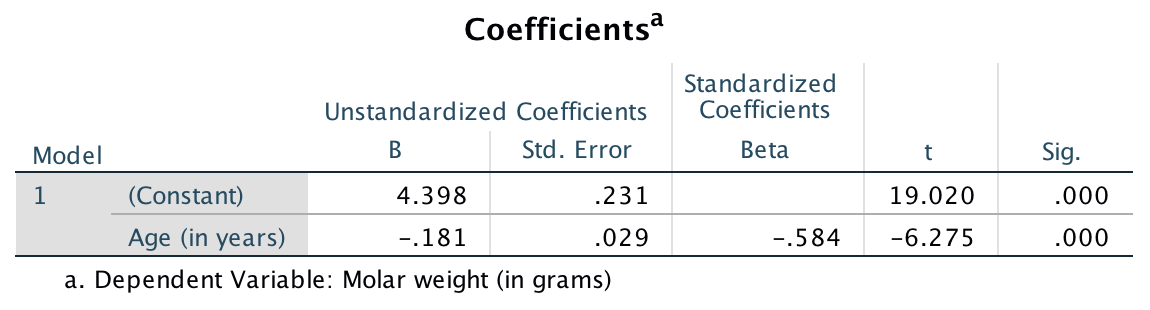
FIGURE 35.4: SPSS output for the red-deer data
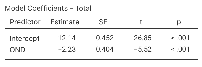
FIGURE 35.5: jamovi output for the cyclone data