35.12 Exercises

Selected answers are available in Sect. D.32.

Exercise 35.1 In wastewater treatment facilities, air from biofiltration is passed through a membrane and dissolved in water, and is transformed into harmless byproducts (Chitwood and Devinny 2001; Devore and Berk 2007). The removal efficiency $y$ (in %) may depend on the inlet temperature (in $^\circ$C; $x$). The RQ is

In treating biofiltation wastewater, how does the removal efficiency depend on the inlet temperature?

Using the scatterplot (Fig. 35.15) and software output (Fig. 35.16 (jamovi); Fig. 35.17 (SPSS)), answer these questions.

1. Write down the value of the slope ($b_1$) and $y$-intercept ($b_0$).
2. Write down the regression equation.
3. Interpret the slope ($b_1$).
4. Test for a relationship in the population, by first writing the hypotheses.
5. Write down the $t$-score and $P$-value from the software output.
6. Determine an approximate 95% CI for the population slope $\beta_1$.
7. Write a conclusion.

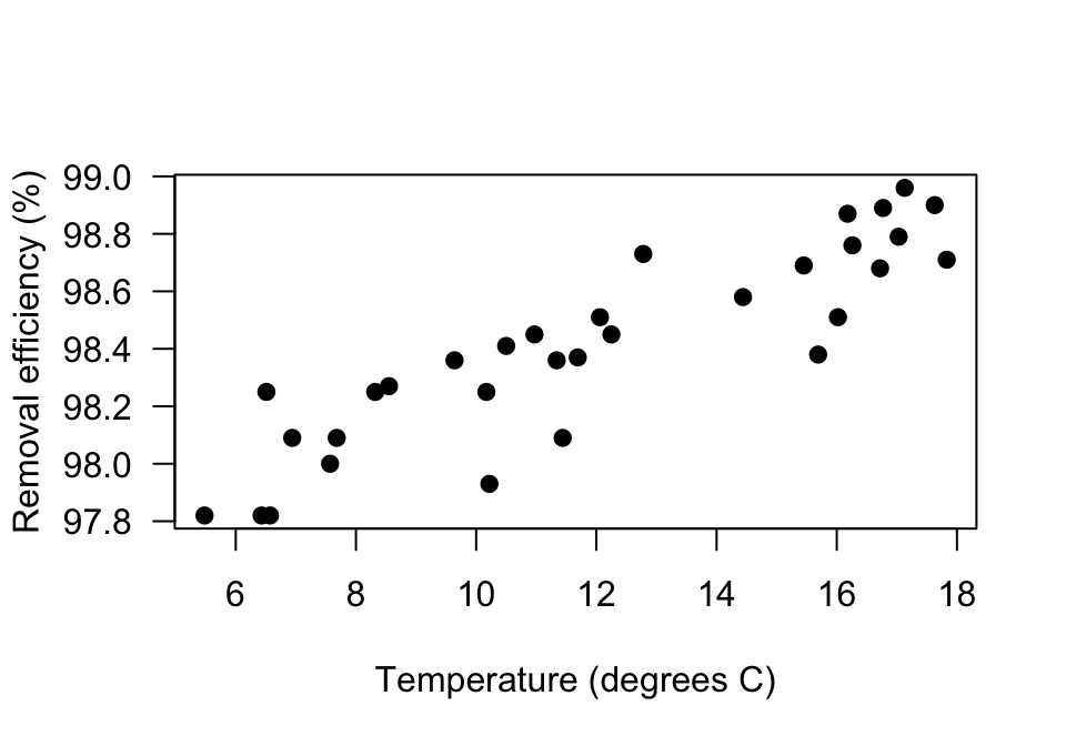
FIGURE 35.15: The relationship between removal efficiency and inlet temperature

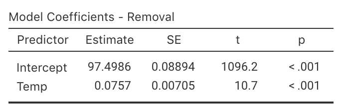
FIGURE 35.16: jamovi regression output for the removal-efficiency data

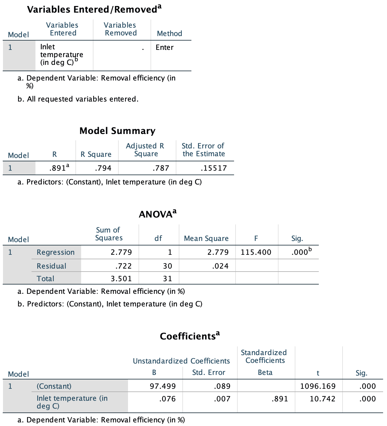
FIGURE 35.17: SPSS regression output for the removal-efficiency data

Exercise 35.2 A study (Myers (1990), p. 75) of American footballers measured the right-leg strengths $x$ of 13 players (using a weight lifting test), and the distance $y$ they punt a football (with their right leg).

1. Use the plot (Fig. 35.18) to guess of the values of the intercept and slope.
2. Using the jamovi output (Fig. 35.19), write down the value of the slope ($b_1$) and $y$-intercept ($b_0$).
3. Hence write down the regression equation.
4. Interpret the slope ($b_1$).
5. Write the hypotheses for testing for a relationship in the population
6. Write down the $t$-score and $P$-value from the output.
7. Determine an approximate 95% CI for the population slope $\beta_1$.
8. Write a conclusion.

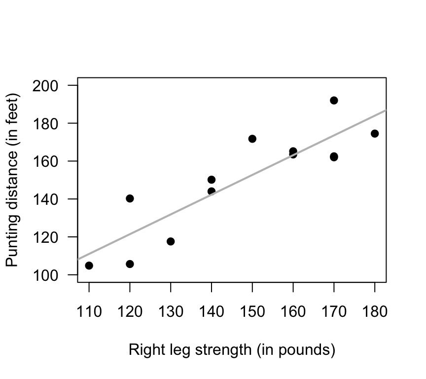
FIGURE 35.18: Punting distance and right leg strength

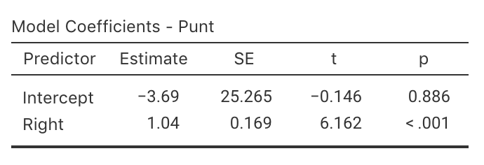
FIGURE 35.19: jamovi regression output for the punting data

Exercise 35.3 A study (Amin and Mahmood-ul-Hasan 2019) of gas engines measured the throttle angle ($x$) and the manifold air pressure ($y$) as a fraction of the maximum value.

1. The value of $r$ is given in the paper as $0.972986604$. Comment on this value, and what it means.
2. Comment on the use of a regression model, based on the scatterplot (Fig. 35.20).
3. The authors fitted the following regression model: $y = 0.009 + 0.458x$. Identify errors that the researchers have made when giving this regression equation (there are more than one).
4. Critique the researchers’ approach.

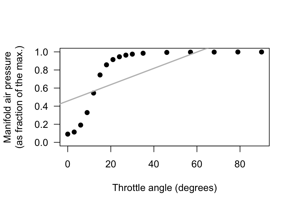
FIGURE 35.20: Manifold air pressure plotted against throttle angle for an internal-combustion gas engine

Exercise 35.4 A study of hot mix asphalt (Panda et al. 2018) created $n=42$ samples of asphalt and measured the volume of air voids and the bitumen content by weight (Fig. 35.21). Use the software output (Fig. 35.22) to answer these questions.

1. Write down the regression equation.
2. Interpret what the regression equation means.
3. Perform a test to determine is there is a relationship between the variables.
4. Predict the mean percentage of air voids by volume when the percentage bitumen is 5.0%. Do you expect this to be a good prediction? Why or why not?
5. Predict the mean percentage of air voids by volume when the percentage bitumen is 6.0%. Do you expect this to be a good prediction? Why or why not?

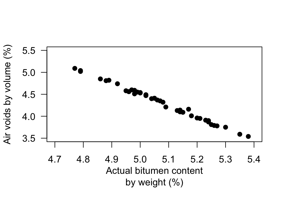
FIGURE 35.21: Air voids in bitumen samples

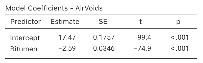
FIGURE 35.22: jamovi regression output for the bitumen data

Exercise 35.5 A study of $n=31$ people on the use of sunscreen (Heerfordt et al. 2018) explored the relationship between the time (in minutes) spent on sunscreen application $x$ and the amount (in grams) of sunscreen applied ($y$). The fitted regression equation was $\hat{y} = 0.27 + 2.21x$.

1. Interpret the meaning of $b_0$ and $b_1$. Do they seems sensible?
2. According to the article, a hypothesis for testing $\beta_0$ produced a $P$-value much larger than $0.05$. What does this mean?
3. If someone spent 8 minutes applying sunscreen, how much sunscreen would you predict that they used?
4. The article reports that $R^2=0.64$. Interpret this value.
5. What is the value of the correlation coefficient?

Exercise 35.6 One study (Bhargava et al. 1985) stated:

In developing countries […] logistic problems prevent the weighing of every newborn child. A study was performed to see whether other simpler measurements could be substituted for weight to identify neonates of low birth weight and those at risk.

— Bhargava et al. (1985), p. 1617

The relationship between infant chest circumference (in cm) $x$ and birth weight (in grams) $y$ was given as:

$$\hat{y} = -3440.2403 + 199.2987x.$$ The correlation coefficient was $r = 0.8696$ with $P < 0.001$.

1. Based on the regression equation only, could chest circumference be used as a useful predictor of birth weight? Explain.
2. Based on the correlation information only, could chest circumference be used as a useful predictor of birth weight? Explain.
3. Interpret the intercept and the slope of the regression equation.
4. What units of measurement are the intercept and slope measured in?
5. Predict the birth weight of an infant with a chest circumference of 30cm.
6. Critique the way in which the regression equation and correlation coefficient are reported.

References

Amin AA, Mahmood-ul-Hasan K. Robust active fault-tolerant control for internal combustion gas engine for air–fuel ratio control with statistical regression-based observer model. Measurement and Control. 2019;0020294018823031.

Bhargava SK, Ramji S, Kumar A, Mohan MAN, Marwah J, Sachdev HP. Mid-arm and chest circumferences at birth as predictors of low birth weight and neonatal mortality in the community. BMJ. British Medical Journal Publishing Group; 1985;291(6509):1617–9.

Chitwood DE, Devinny JS. Treatment of mixed hydrogen sulfide and organic vapors in a rock medium biofilter. Water Environment Research. Water Environment Federation; 2001;73(4):426–35.

Devore JL, Berk KN. Modern mathematical statistics with applications. Thomson Higher Education; 2007.

Heerfordt IM, Torsnes LR, Philipsen PA, Wulf HC. Photoprotection by sunscreen depends on time spent on application. Photodermatology, Photoimmunology & Photomedicine. Wiley Online Library; 2018;34(2):117–21.

Myers RH. Classical and modern regression with applications. second. Duxbury; 1990.

Panda RP, Das SS, Sahoo PK. Relation between bitumen content and percentage air voids in semi dense bituminous concrete. Journal of The Institution of Engineers (India): Series A. 2018;99(2):327–32.

---

Copyright © Peter K. Dunn, 2021