35.6 Hypothesis testing
35.6.1 Introduction
The regression line is computed from the sample, assuming a linear relationship actually exists in the population. The (unknown) regression line in the population is
\[ \hat{y} = {\beta_0} + {\beta_1} x. \] From the sample, the estimate of the population regression line (Appendix C) is
\[ \hat{y} = {b_0} + {b_1} x. \] That is, the intercept in the population is \(\beta_0\) (estimated by \(b_0\)), and the slope in the population is \(\beta_1\) (estimated by \(b_1\)). The sample can be used to ask questions about the population regression coefficients. As usual, the sample values can vary from sample to sample (and so have a sampling distribution).
Usually questions are asked about the slope, because the slope explains the relationship between the two variables (Sect. 35.5).
35.6.2 Hypotheses: Assumption
The null hypothesis is the usual ‘no relationship’ hypothesis. In this context, ‘no relationship’ means that the slope is zero (Sect. 35.5.2). Hence, the null hypotheses (about the population) is:
- \(H_0\): \(\beta_1 = 0\).
This hypothesis proposes that \(b_1\) is not zero because of sampling variation. As part of the decision-making process, the null hypothesis is initially assumed to be true.
For the red deer data (Sect. 33.2), determining if a relationship exists between the age of the deer, and the weight of their molars, would test these hypotheses:
- \(H_0\): \(\beta_1 = 0\);
- \(H_1\): \(\beta_1 \ne 0\)
The parameter is \(\beta\), the population slope for the regression equation predicting molar weight from age.
The alternative hypothesis is two-tailed, based on the RQ.
35.6.3 Sampling distribution: Expectation
Assuming the null hypothesis is true (that \(\beta_1=0\)), we can describe what values the sample slope \(b_1\) are expected to take, through sampling variation. The variation in the sample slope from sample to sample can be described (Fig. 35.6) using:
- an approximate normal distribution,
- with a mean of \(\beta_1 = 0\) (from \(H_0\)), and
- a standard deviation, called the standard error of the slope, of \(\text{s.e.}(b_1)\).
The standard error is found using software (jamovi: Fig. 35.7; SPSS: Fig. 35.8).
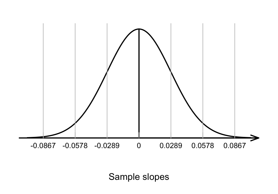
FIGURE 35.6: The distribution of sample slope for the red deer data, if the population slope is 0
35.6.4 The test statistic: Observation
The observed sample slope was \(b_1 = -0.181\). The test statistic would be found using the usual approach:
\[\begin{align*} t &= \frac{ b_1 - \beta_1}{\text{s.e.}(b_1)} \\ &= \frac{-0.181 - 0}{0.0289} = -6.27, \end{align*}\] where the values of \(b_1\) and \(\text{s.e.}(b_1)\) are taken from the software output. The \(t\)-score is also reported by the software.
35.6.5 \(P\)-value: Consistency with assumption
To determine if the statistic is consistent with the null hypothesis, the \(P\)-value can be approximated using the 68–95–99.7 rule, or taken from software output (jamovi: Fig. 35.7; SPSS: Fig. 35.8). Using software, the \(P\)-value is \(P<0.001\). The sample presents very strong evidence that the slope in the population between age of the deer and molar weight is not zero.
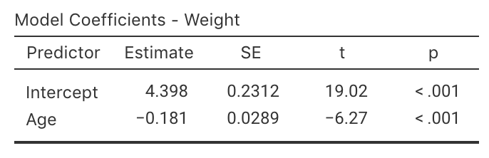
FIGURE 35.7: jamovi output for the red-deer data
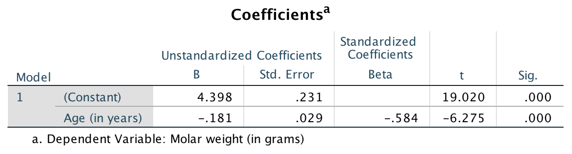
FIGURE 35.8: SPSS output for the red-deer data