13.2 Computing the average value

The average (or location, or centre, or typical value) for quantitative sample data can be described in many ways; the two most common ways are:
- the sample mean (or sample arithmetic mean), which estimate the population mean; and
- the sample median, which estimates the population median.
In both cases, the population parameter is estimated by a sample statistic. Understanding whether to use the mean or median is important.

Think 13.1 (Difference between averages) Consider the daily river flow volume (called ‘streamflow’) at the Mary River from 01 October 1959 to 17 January 2019, summarised by month in Table 13.1 (from Queensland DNRM).
The ‘average’ daily streamflow in February could be quoted using either the mean or the median; but the two give very different values for the ‘average’:
- the mean daily flow is 1123.2ML.
- the median daily flow is 146.1ML.
| Month | Mean | Median |
|---|---|---|
| Jan | 849.3 | 71.3 |
| Feb | 1123.2 | 146.1 |
| Mar | 793.9 | 194.9 |
| Apr | 622.5 | 141.7 |
| May | 348.4 | 118.4 |
| Jun | 378.7 | 83.6 |
| Jul | 259.3 | 68.8 |
| Aug | 108.6 | 55.5 |
| Sep | 100.9 | 48.0 |
| Oct | 151.2 | 37.6 |
| Nov | 186.6 | 45.3 |
| Dec | 330.8 | 64.1 |
13.2.1 Computing the average: The mean
The mean of the population is denoted by \(\mu\), and its value is almost always unknown.
Instead, the mean of the population is estimated by the mean of the sample, which is denoted by \(\bar{x}\) (an \(x\) with a line above it). In this context, the unknown parameter is \(\mu\), and the statistic is \(\bar{x}\). The sample mean is used to estimate the population mean.
The Greek letter \(\mu\) is pronounced ‘myoo,’ as in music.
The symbol \(\bar{x}\) is pronounced ‘ex-bar.’
Example 13.2 (A small data set to work with) To demonstrate ideas, consider a small data set for answering this descriptive RQ:
For mature Jersey cows, what is the average percentage butterfat in their milk?
The population is ‘milk from Jersey cows,’ and an estimate of the population mean percentage butterfat is sought. The population mean is denoted by \(\mu\).
Clearly, milk from every Jersey cow cannot be studied; a sample is studied (Sokal and Rohlf 1995; Hand et al. 1996): The unknown population mean is estimated using the sample mean (\(\bar{x}\)). Measurements were taken from milk from 10 cows, in percentages (Table 13.2).| 4.8 | 5.2 | 5.2 | 5.4 | 5.2 |
| 6.5 | 4.5 | 5.7 | 4.8 | 5.2 |
The sample mean is what people usually think of as the ‘average.’ The sample mean is actually the ‘balance point’ of the observations. The animation below shows how the mean acts as the balance point. Alternatively, the mean is the value such that the positive and negative distances of the observations from the mean add to zero , as shown in the animation below. Both of these explanations seem reasonable for identifying the ‘average’ of the data.
To find the value of the sample mean:
- Add (shown using the symbol \(\sum\)) all the observations (denoted by \(x\)); then
- Divide by the number of observations (denoted by \(n\)).
In symbols: \[ \bar{x} = \frac{\sum x}{n}. \] This means to add up (indicated by \(\sum\)) the observations (denoted by \(x\)), then divide by the size of the sample (denoted by \(n\)).
| 484 | 492 | 436 | 464 |
| 478 | 444 | 398 | 476 |
Software and calculators often produce numerical answers to many decimal places, some of which may not be meaningful or useful. A useful rule-of-thumb is to round to one or two more significant figures than the original data.
For example, the butterfat data are given to one decimal place. The sample mean weight can be given to two decimal places: \(\bar{x}=5.25\)%.13.2.2 Computing the average: The median
The median is a value separating the larger half of the data from the smaller half of the data. In a data set with \(n\) values, the median is ordered observation number \(\displaystyle \frac{n+1}{2}\). The median is:
- not equal to \(\displaystyle \frac{n+1}{2}\).
- not halfway between the minimum and maximum values in the data.
Most calculators cannot find the median.
| 4.5 | 4.8 | 4.8 | 5.2 | 5.2 |
| 5.2 | 5.2 | 5.4 | 5.7 | 6.5 |
Think 13.5 (Medians) A study of eyes (Ehlers 1970) aimed to estimate the average thickness of eyes affected by glaucoma.
Using the collected data (Table 13.3), estimate the population median corneal thickness. What is the population median?With \(n=8\) observations, the median is ordered observation number \((8+1)/2 = 4.5\), halfway between ordered observation numbers 4 and 5. After sorting into increasing order, the two middle numbers (the 4th and 5th) are 464 and 476. The median could be any number between 464 and 476, but the usual answer would be that the median is \((464 + 476)/2 = 470\).
The sample median is 470 microns; the value of the population median remains unknown.To clarify:
- If the sample size \(n\) is odd, the median is the middle number when the observations are ordered.
- If the sample size \(n\) is even (such as in Think 13.5), the median is halfway between the two middle numbers, when the observations are ordered.
Some software uses different rules when \(n\) is even.
13.2.3 Which average to use?
Consider again estimating the average daily streamflow at the Mary River (Bellbird Creek) during February (Table 13.1): The mean daily streamflow is 1123.2ML, and the median daily streamflow is 146.1ML. Which is the ‘best’ average to use?
A dot chart of the daily stream flow (Fig. 13.2) shows that the data are very highly right-skewed, with many very large outliers: the maximum value is 156586.4ML, more than one hundred times larger than the mean of 1123.2ML). In fact, about 86% of the observations are less than the mean. In contrast, about 50% the values are less than the median (by definition). For these data, the mean is hardly a central value…
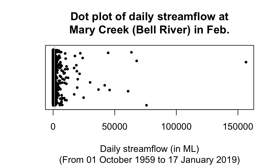
FIGURE 13.2: A dot plot of the daily streamflow at Mary River from 1960 to 2017, for February. The vertical grey line is the mean value. Many large outliers exist, so the data near zero are all squashed together
The streamflow data are very highly skewed (to the right), which is important and relevant:
- Means are best used for approximately symmetric data: the mean is influenced by outliers and skewness.
- Medians are best used for data that are skewed or contain outliers: the median is not influenced by outliers and skewness.
Means tend to be too large if the data contains large outliers or severe right skewness, and too small if the data contains small outliers or severe left skewness.
For the Mary River data, the large outliers—and the fact that they are so extreme and abundant—result in the mean being substantially influenced by the outliers, which explains why the mean is much larger than the median. The median is the better measure of average for these data.
The mean is generally used if possible (for practical and mathematical reasons), and is the most commonly-used measure of location. However, the mean is influenced by outliers and skewness; the median is not influenced by outliers and skewness. The mean and median are similar in approximately symmetric distributions. Sometimes, quoting both the mean and the median may be appropriate.
Think 13.6 (Which average to use) An engineering study (Hald 1952) was studying a new building material to determine the average permeability time.
The time (in seconds) taken for water to permeate \(n=81\) pieces of material. Using a histogram of the data (Fig. 13.3), estimate the value of the population mean and median. Which would be best to use (for example, to quote an average permeability time on a specification sheet)?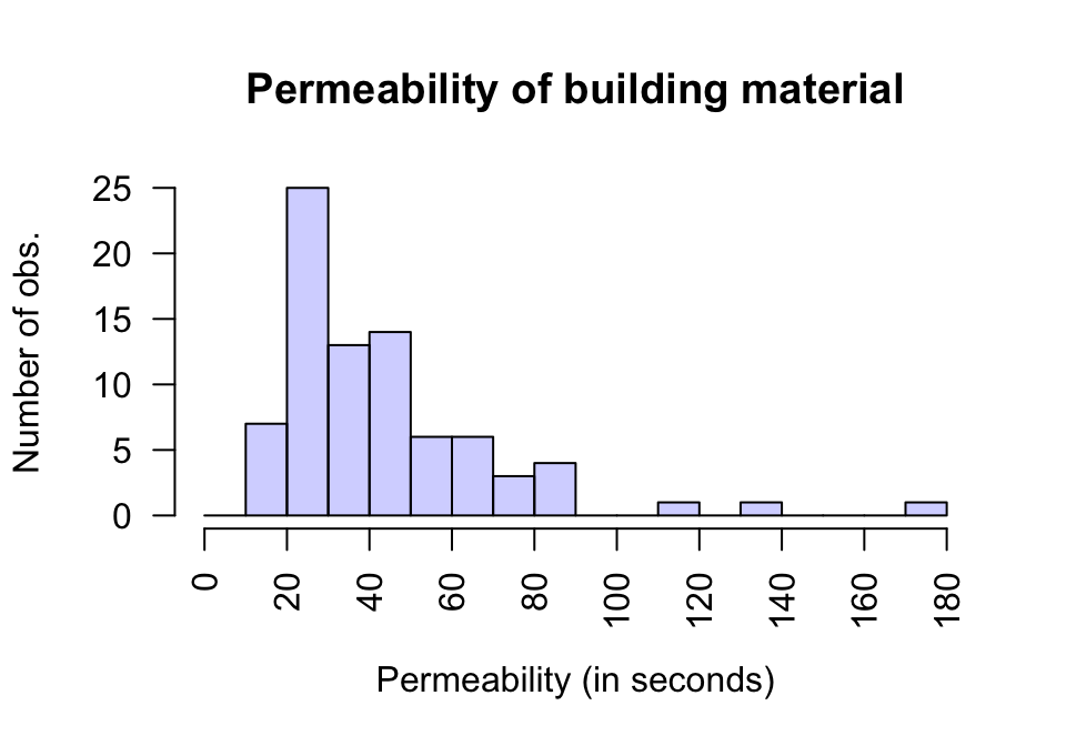
FIGURE 13.3: A histogram of the permeability of a type of building material