33.2 Two quantitative variables: Graphical summaries

For the red deer data, both variables are quantitative, so the appropriate graphical summary (Sect. 12.5) is a scatterplot (Fig. 33.2).

In the graph, the response variable is graphed on the vertical axis, and denoted \(y\); the explanatory variable is graphed on the horizontal axis, and denoted \(x\). The explanatory variable (potentially) influences the response variable, so in this example:

The explanatory variable (\(x\)) is the age of the deer (in years), and
The response variable (\(y\)) is the weight of molars (in grams).

In other words, the age of the deer would seem likely to influence the weight of the molars. (In some cases, it doesn’t matter which is \(x\) and which is \(y\), such as exploring the relationship between height and weight of red deer.)

Note that each row in the data set (and each point on the scatterplot) correspond to a single deer (the deer are the units of analysis), and two different variables (age; molar weight) are measured on each deer.

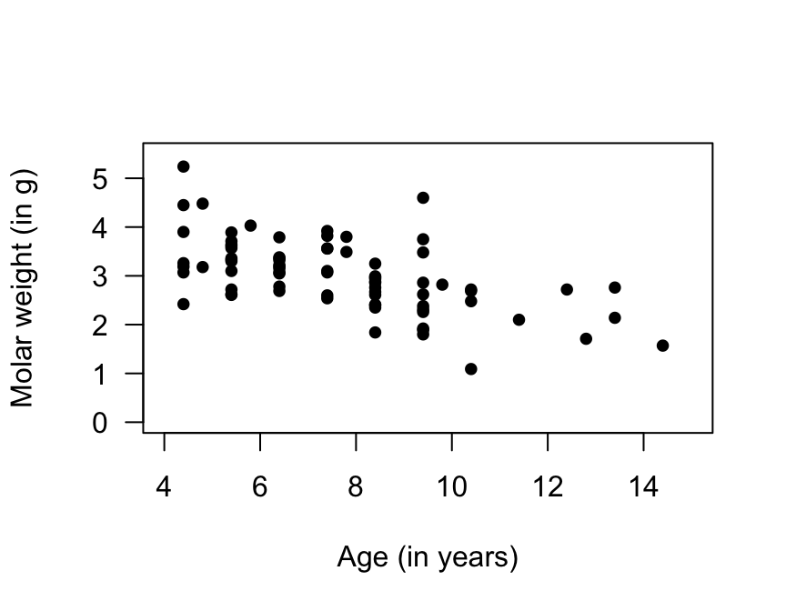
FIGURE 33.2: Molar weight verses age for the red deer data