20.6 Statistical validity conditions
The histogram in Sect. 20.1, shows the proportion of \(n=25\) rolls that were even for many samples; it has an approximate normal distribution. Because of this, the 68–95–99.7 rule could be used to form the approximate 95% CIs.
However, the distribution of the sample proportions only looks like a normal distribution under certain conditions. Certain conditions must be true for the calculations to be sensible, or statistically valid.

Example 20.4 (Statistical validity analogy) Suppose your doctor asks you to get a blood test, after fasting (refraining from eating) for 12 hours before your blood test.
After leaving the doctor, you proceed to a restaurant for dinner. You start the next day with a hearty breakfast, have lunch at a beach-side cafe, and then go for your blood test. Your blood is extracted, the blood is analysed in the pathology lab, and your doctor is emailed the results of the blood test.
However, since you did not fast as required, the results may or may not be valid. The doctor can still learn something… but not as much as if you had followed the instructions.
Similarly, if the conditions for computing the confidence interval are not met, the results may be suspect.The statistical validity conditions for creating CI for a single proportion is that:
- the number of individuals in the group of interest must exceed 5, and
- the number of individuals in the group not of interest must exceed 5.
These conditions ensure that the sampling distribution of \(\hat{p}\) has an approximate normal distribution, so that the 68–95–99.7 rule (approximately) applies. If this condition is not met, the sampling distribution may not have normal distribution, so the 68–95–99.7 rule (used to create the CI) maybe inappropriate, and so the CI may also be inappropriate.
In addition to the statistical validity condition, the CI will be:
- internally valid if the study was well designed; and
- externally valid if the the sample is a simple random sample and is internally valid.

Example 20.5 (Energy drinks in Canadian youth) In Example 20.1, the approximate 95% CI was from 0.192 to 0.236. This confidence interval for the sample proportion will be statistically valid if:
- the number of youth in the sample who experienced sleeping difficulties exceeds 5; and
- the number of youth in the sample who didn’t experience sleeping difficulties exceeds 5.
The number of youth experiencing sleeping difficulties was 365, which is more than five. The number of youth not experiencing sleeping difficulties was \(1516 - 365 = 1151\), which is also more than five. Hence, the CI is statistically valid.
In addition, the CI will be internally valid if the study was well designed, and will be externally valid if the sample is a simple random sample from the population and is internally valid.Example 20.6 (Statistical validity) Consider an artificial situation to estimate the proportion of die rolls that show as a one. The population proportion (using the classical approach to probability) is 1/6, or about 0.167.
If we repeatedly rolled a die in sets of \(n=20\) rolls, say 5000 times, the proportion of rolls that showed as one could be recorded for each set of 20 rolls. Then, a histogram of the sample proportions could be produced. Using a computer to simulate this, a histogram of the sample proportions is shown in the top panel of Fig. 20.5. The normal distribution does a poor job of describing the sampling distribution (the distribution is not even symmetric). The statistical validity conditions do not seem satisfied.
Alternatively, we could repeatedly roll a die in sets of \(n=60\) rolls, say 5000 times, and record the proportion of rolls that show as one for each set of 60 rolls. Then, a histogram of the proportion of ones for those sets of 60 rolls could be produced. Using a computer to simulate this, a histogram of these proportions is shown in the bottom panel of Fig. 20.5. The normal distribution does a reasonable job of describing the sampling distribution. The statistical validity conditions seem satisfied.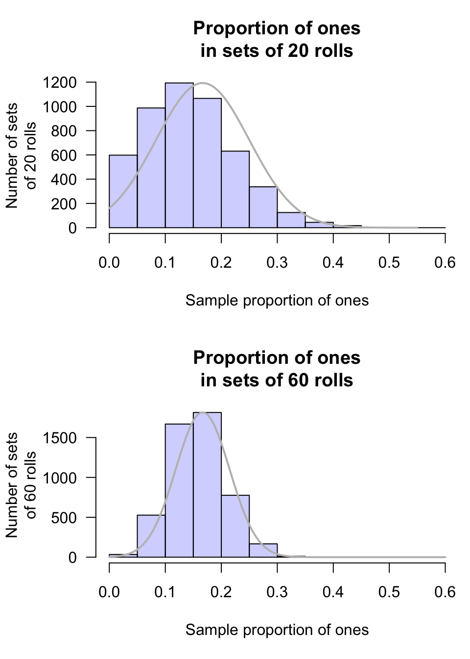
FIGURE 20.5: The sampling distribution of the proportion of ones rolled, for sets of 20 rolls (top panel) and sets of 60 rolls (bottom panel)