27.10 Example: Recovery times

Seventeen patients were treated for medial collateral ligament (MCL) and anterior cruciate ligament (ACL) tears using a new treatment method (Altman 1991; Nakamura et al. 2000). The current existing treatment has an average recovery time of 15 days. The RQ is:
For patients with this type of injury, does the new treatment method lead to shorter mean recovery times?
The parameter is \(\mu\), the population mean recovery time.
The hypotheses (Step 1: Assumption) about the parameter are, from the RQ:
- \(H_0\): \(\mu=15\) (the population mean is \(15\), but \(\bar{x}\) is not \(15\) due to sampling variation): This is the initial assumption.
- \(H_1\): \(\mu<15\) (\(\mu\) is not \(15\); it really does produce shorter recovery times, on average).
This test is one-tailed: the RQ only asks if the new method produces shorter recovery times.
The evidence (Table 27.2) can be summarised numerically, using software or (since the data set is small) a calculator. Either way, \(\bar{x} = 13.29\) and \(s=8.887\).
| 14 | 18 | 12 | 10 | 8 | 28 | 24 | 3 | 9 |
| 9 | 26 | 0 | 4 | 21 | 24 | 2 | 14 |
If the null hypothesis is true (and \(\mu=15\)), the values of the sample mean that are likely to occur through sampling variation can be described (Step 2: Expectation). The sample means are likely to vary with an approximate normal distribution (under certain assumptions), with mean \(\mu=15\) and a standard deviation of
\[ \text{s.e.}(\bar{x}) = \frac{s}{\sqrt{n}} = \frac{8.887}{\sqrt{17}} = 2.155. \] This describes what values of \(\bar{x}\) we should expect in the sample if the mean recovery time \(\mu\) really was 15 days (Fig. 27.10).
The sample mean is \(\bar{x} = 13.29\), so the \(t\)-score to determine where the sample mean is located (Step 3: Observation), relative to what is expected, is
\[ t = \frac{\bar{x} - \mu}{\text{s.e.}(\bar{x})} = \frac{13.29 - 15}{2.155} = -0.79. \] Software could also be used (jamovi: Fig. 27.8; SPSS: Fig. 27.9), but in either case, \(t = -0.79\).
A \(z\)-score of \(-0.79\) is not unusual, and (since \(t\)-scores are like \(z\)-scores) this \(t\)-score is not unusual either (Step 4: Consistency). The \(P\)-value in the jamovi output or SPSS output confirms this: the two-tailed \(P\)-value is \(0.440\), so the one-tailed \(P\)-value is \(0.440\div 2 = 0.220\).
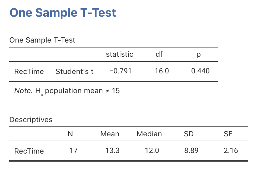
FIGURE 27.8: jamovi output for the \(t\)-test for the recovery-times data
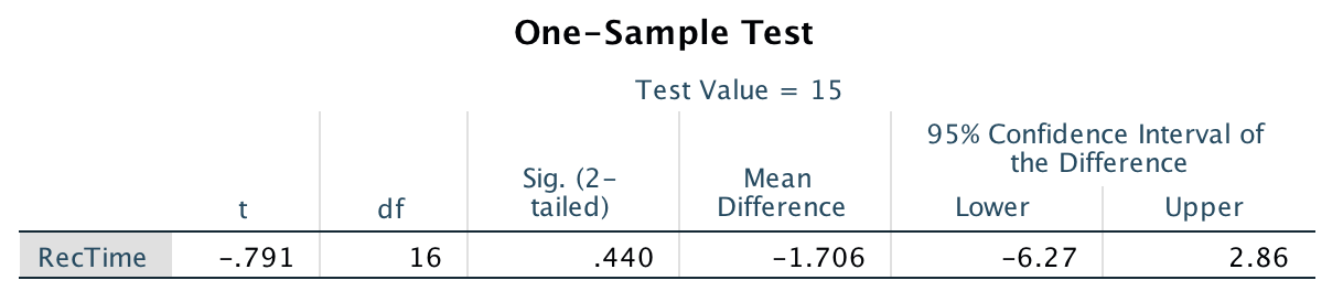
FIGURE 27.9: SPSS output for the \(t\)-test for the recovery-times data
This ‘large’ \(P\)-value suggests that a sample mean of 13.29 could reasonably have been observed just through sampling variation: there is no evidence to support the alternative hypothesis \(H_1\). If \(\mu\) really was 15, then about 22% of the time \(\bar{x}\) would be less than 13.29 just through sampling variation alone.
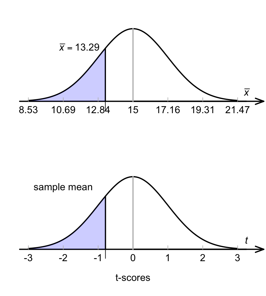
FIGURE 27.10: The sampling distribution for the recovery-times data
To summarise:
- Step 1 (Assumption):
- \(H_0\): \(\mu=15\), the initial assumption;
- \(H_1\): \(\mu<15\) (note: one-tailed)
- Step 2 (Expectation): The sample means will vary, and this sampling variation is described by an approximate normal distribution with mean \(15\) and standard deviation \(\text{s.e.}(\bar{x}) = 2.155\).
- Step 3 (Observation): \(t = -0.791\).
- Step 4 (Consistency?): The one-tailed \(P\)-value is \(0.220\): The data are consistent with \(H_0\), so there is no evidence to support the alternative hypothesis.
To write a conclusion, include an answer to the question, evidence leading to the conclusion, and some sample summary information:
No evidence exists in the sample (one sample \(t = -0.79\); one-tailed \(P=0.220\)) that the population mean recovery time is less than 15 days (mean 13.29 days; \(n=17\); 95% CI from 8.73 to 17.86 days) using the new treatment method.
(The CI is found using the ideas in Sect. 22.3, or manually.) Notice the wording: The new method may be better, but no evidence exists of this in the sample. The onus is on the new method to demonstrate that it is better than the current method.
The sample size is small (\(n=17\)), so the test may not be statistically valid (but the \(P\)-value is so large that it probably won’t affect the conclusions).