25.9 Exercises
Selected answers are available in Sect. D.24.
Exercise 25.1 A prospective observational study (Wallace et al. 2017) compared the heights of scars from burns received in Western Australia (Table 25.8). jamovi was used to analyse the data (Fig. 25.12).
- Compute the odds of having a smooth scar (that is, height is 0mm) for women.
- Compute the odds of having a smooth scar (that is, height is 0mm) for men.
- Compute the odds ratio of having a smooth scar, comparing women to men.
- Interpret what this odds ratio means.
- Sketch a suitable graph to display the data.
- Construct an appropriate numerical summary table for the data.
- Write down the CI.
- Carefully interpret what this CI means.
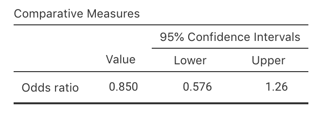
FIGURE 25.12: jamovi output for the scar-height data
| Women | Men | |
|---|---|---|
| Scar height 0mm (smooth) | 99 | 216 |
| Scar height more than 0mm, less than 1mm | 62 | 115 |
Exercise 25.2 A study of ear infections in Sydney swimmers (Smyth 2010) recorded whether people reported an ear infection or not, and where they usually swam.
The SPSS output is shown in Fig. 25.13. Explain carefully the meaning of the OR and the corresponding CI.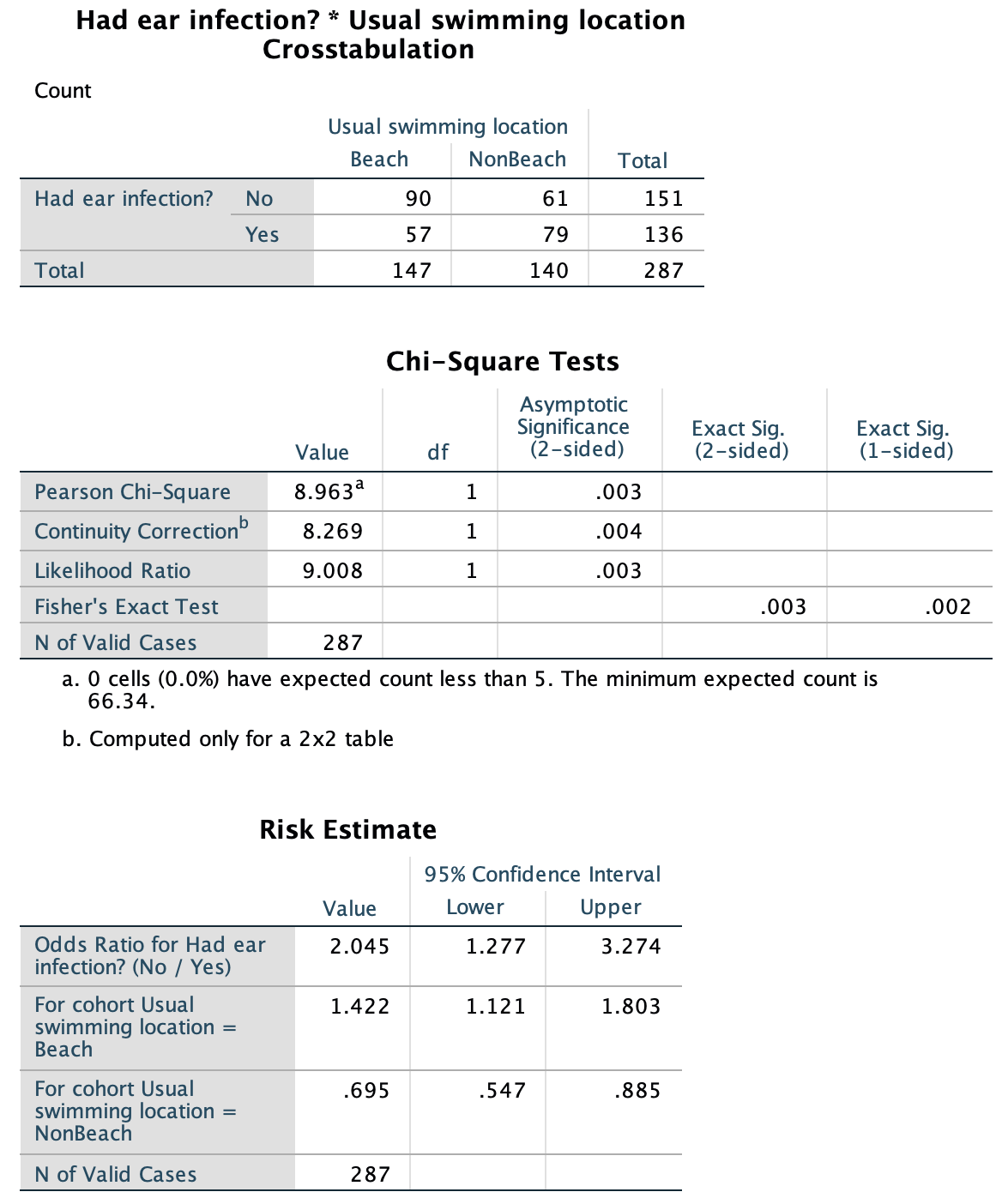
FIGURE 25.13: SPSS output for the ear-infection data
Exercise 25.3 A study of turbine failures (Nelson 1982; Myers et al. 2002) ran 73 turbines for around 1800 hours, and found that seven developed fissures (small cracks). They also ran a different set of 42 turbines for about 3000 hours, and found that nine developed fissures.
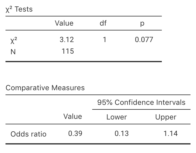
FIGURE 25.14: jamovi output for the turbine data: output
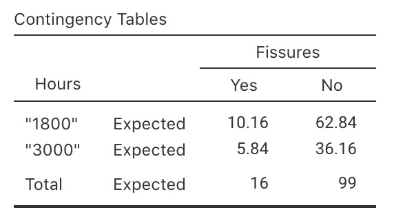
FIGURE 25.15: jamovi output for the turbine data: expected counts
Exercise 25.4 The Southern Oscillation Index (SOI) is a standardised measure of the air pressure difference between Tahiti and Darwin, and is related to rainfall in some parts of the world (Stone et al. 1996), and especially Queensland (Stone and Auliciems 1992; Dunn 2001).
The rainfall at Emerald (Queensland) was recorded for Augusts between 1889 to 2002 inclusive (Dunn and Smyth 2018), where the monthly average SOI was positive, and when the SOI was non-positive (that is, zero or negative), as shown in Table 25.9.
Using the jamovi output in Fig. 25.16:
- Find a 95% CI for the OR.
- Carefuly explain what this OR means.
| Non-positive SOI | Positive SOI | |
|---|---|---|
| No rainfall recorded | 14 | 7 |
| Rainfall recorded | 40 | 53 |
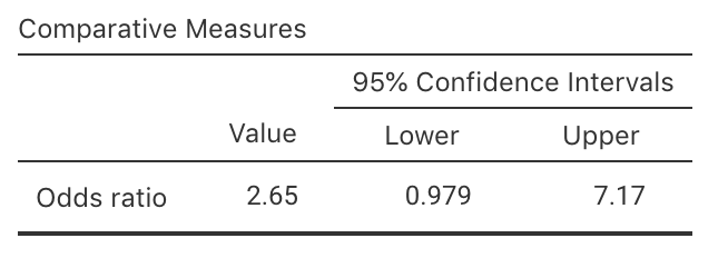
FIGURE 25.16: jamovi output for the Emerald-rain data
Exercise 25.5 A research study conducted in Brisbane (Dexter et al. 2019) recorded the number of people at the foot of the Goodwill Bridge, Southbank, who wore sunglasses and hats between 11:30am to 12:30pm. Table 25.10 records the number of females and males wearing hats.
Using the SPSS output in Fig. 25.17, find a 95% CI for the OR, and carefully explain what OR this CI applies to. Also, construct the numerical summary table.
| No hat | Hat | |
|---|---|---|
| Male | 307 | 79 |
| Female | 344 | 22 |
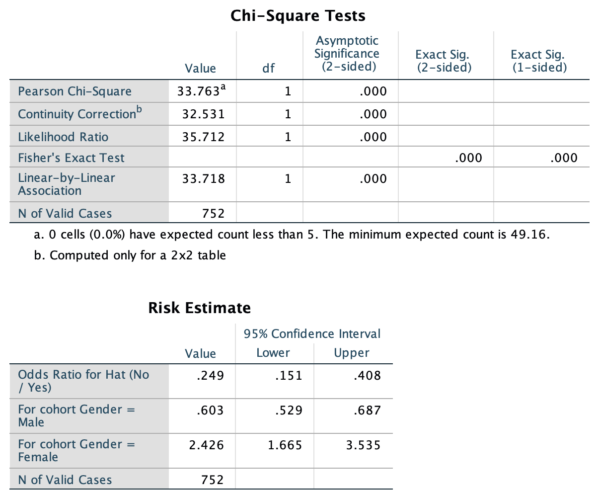
FIGURE 25.17: SPSS output for the hats data