20.4 Confidence intervals: Unknown proportion
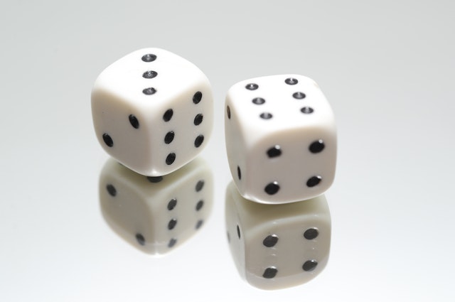
Suppose thousands of people rolled a die 25 times, and each person found \(\hat{p}\) for their sample, and hence computed the CI for their sample of 25 rolls.
Every sample of 25 rolls could produce a different estimate \(\hat{p}\), and so a different value for \(\text{s.e.}(\hat{p})\), and hence a different 95% CI. However, about 95% of these thousands of confidence intervals from those thousands of repetitions would straddle the true proportion \(p\).
Since we usually don’t know the value of \(p\), and we usually only have one sample (and hence one CI), in general we never know whether the single CI computed from our single sample straddles \(p\) or not.
Again, consider letting the computer simulate the situation. Suppose the process of recording the sample proportion of even numbers in \(n=25\) rolls is repeated 50 times, and for each of those 50 sets of 25 rolls a CI is produced (see the animation below).
Most of those CIs straddle the population proportion of \(p=0.5\) (shown as solid lines)… but some do not (shown as dashed lines). Of course, since the value of \(p\) is usually unknown, we never know if our CI contains \(p\) or not.
Definition 20.3 (Confidence interval) A confidence interval is an interval in which the population parameter is likely to be contained, if we found many samples the same way.
If a 95% confidence interval (or CI) is computed from each sample, about 95% of the CIs would straddle the parameter of interest. This interval is called a confidence interval.In general, a CI for the population proportion \(p\) is found using
\[ \hat{p} \pm ( \text{multiplier} \times \text{s.e.}(\hat{p})), \] where the multiplier is 2 for an approximate 95% CI (based on the 68–95–99.7 rule).
Definition 20.4 (Confidence interval for \(p\)) A confidence interval (CI) for the unknown value of the parameter \(p\) is \[\begin{equation} \hat{p} \pm ( \text{multiplier} \times \text{s.e.}(\hat{p})), \tag{20.4} \end{equation}\] where
\[ \text{s.e.}(\hat{p}) = \sqrt{\frac{ \hat{p} \times (1 - \hat{p}) }{n}} \] is the standard error of \(\hat{p}\), \(\hat{p}\) is the sample proportion, and \(n\) is the sample size. For an approximate 95% CI, the multiplier is 2.In general, higher confidence levels means wider intervals: To be more confident that the interval straddles the unknown value of \(p\), wider intervals are needed (Fig. 20.4) to cover more possibilities.
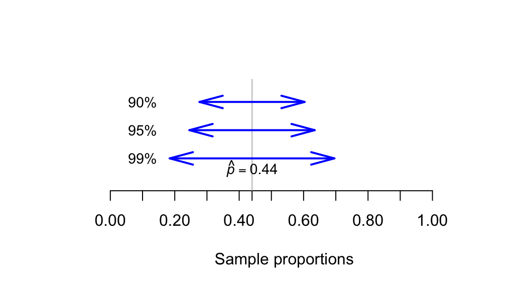
FIGURE 20.4: To have greater confidence that the interval will straddle the population proportion, the interval needs to be wider

Example 20.1 (Energy drinks in Canadian youth) A study of young Canadians aged 12–24 (Hammond et al. 2018) found that 365 of the 1516 respondents reported sleeping difficulties after consuming energy drinks.
The unknown parameter is \(p\), the population proportion of young Canadians reporting sleeping difficulties.
The sample proportion reporting sleeping difficulties after consuming energy drinks is \(\hat{p} = 365/1516 = 0.241\). As usual, the sample proportion would vary from one sample of size \(n=1516\) to another; sampling variation exists. The standard error (Definition 20.4) quantifies how much the sample proportion is likely to vary from sample to sample:
\[\begin{align*} \text{s.e.}(\hat{p}) &= \sqrt{\frac{\hat{p}\times(1-\hat{p})}{n}}\\ &= \sqrt{\frac{0.241 \times (1-0.241)}{1516}} = 0.01098449, \end{align*}\] or about \(0.011\). So, in samples of size 1516, the approximate 95% CI (Definition 20.4) is between
- \(0.241 - (2\times 0.01098449) = 0.2190\) and
- \(0.241 + (2\times 0.01098449) = 0.2627\).
The approximate 95% CI is from 0.219 to 0.263.
This CI may or may not straddle the population proportion \(p\); it is likely that the interval straddles the value of \(p\). In other words, it is plausible that the sample proportion of \(p=0.241\) may have come from a population with a proportion somewhere between 0.219 and 0.263.
Example 20.2 (Koalas crossing roads) A study of koalas (Dexter et al. 2018) found that 18 of the \(n=51\) koalas studied in a certain area (over 30 months) had crossed at least one road during that time.
The unknown parameter is \(p\), the population proportion of koalas that had crossed at least one road over the 30 months.
The sample proportion having crossed a road is \(\hat{p} = 18/51 = 0.3529\). The standard error (Definition 20.4) is
\[\begin{align*} \text{s.e.}(\hat{p}) &= \sqrt{ \frac{ \hat{p} \times (1 - \hat{p})}{n} }\\ &= \sqrt{ \frac{0.3529 \times (1 - 0.3529)}{51} }\\ &= 0.06692. \end{align*}\] An approximate 95% CI, then, is \(0.3529 \pm (2 \times 0.06692)\), or
\[ 0.3529 \pm 0.1338. \] The margin of error is \(0.1338\).
Computing the ‘plus’ and the ‘minus’ bits, the approximate 95% CI is from 0.219 to 0.487 (after rounding appropriately).
The approximate 95% CI for the population proportion of koalas that crossed at least one road in the last 30 months is from 0.219 to 0.487. That is, it is plausible that the sample proportion of \(\hat{p}=0.3529\) may have come from a population with a proportion somewhere between 0.219 and 0.487.
The research article reports:
This agrees with our calculations.Of the 51 koalas, 18 (35.3%) crossed at least one road. The […] probability of a koala crossing at least one road during the study was 35.3% (95% CI = 22–48%).
— Dexter et al. (2018), p. 70.