20.3 Sampling distribution: Unknown proportion
In the die example (Sect. 20.1), an equation was given for computing the standard error for the sample proportion for samples of size \(n\), when the value of \(p\) was known.
However, usually the value of \(p\) (the parameter) is unknown; after all, the reason for taking a sample is to estimate the unknown value of \(p\). When \(p\) is unknown, the best available estimate can be used, which is \(\hat{p}\). When the value of \(p\) is unknown, the standard error of the sample proportion (written \(\text{s.e.}(\hat{p})\)) is approximately
\[ \text{s.e.}(\hat{p}) = \sqrt{\frac{ \hat{p} \times (1-\hat{p})}{n}}. \]
Definition 20.2 (Sampling distribution of a sample proportion when \(p\) is unknown) When the value of \(p\) is unknown, the sampling distribution of the sample proportion is described by
- an approximate normal distribution,
- centred around the (unknown) mean of \({p}\),
- with a standard deviation (called the standard error of \(\hat{p}\)) of
\[\begin{equation} \text{s.e.}(\hat{p}) = \sqrt{\frac{ \hat{p} \times (1-\hat{p})}{n}}, \tag{20.3} \end{equation}\]
when certain conditions are met, where \(n\) is the size of the sample, and \(\hat{p}\) is the sample proportion.
In general, the approximation gets better as the sample size gets larger.Let’s pretend for the moment that the proportion of even rolls of a fair die is unknown (to demonstrate some points). In this case, an estimate of the proportion of even rolls can be found by rolling a die \(n=25\) times and computing \(\hat{p}\).
Suppose 11 of the \(n=25\) rolls produced an even number, so that \(\hat{p} = 11/25 = 0.44\). Then (from Definition 20.2),
\[ \text{s.e.}(\hat{p}) = \sqrt{ \frac{ 0.44 \times (1 - 0.44)}{25}} = 0.099277. \] (This is very similar to the value of 0.1, the value of the standard error when the value of \(p\) was known; see Eq. (20.2).)
Hence, the sample proportions would vary with an approximate normal distribution (Fig.20.3), centred around the unknown value of \(p\) with a standard deviation of \(\text{s.e.}(\hat{p}) = 0.099277\).
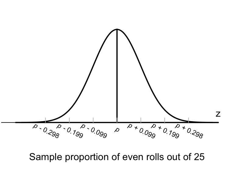
FIGURE 20.3: The normal distribution, showing how the proportion of even rolls varies when a die is rolled 25 times
Using the 68–95–99.7 rule again:
About 95% of the values of \(\hat{p}\) are expected to be between \(p - 0.199\) and \(p + 0.199\).
Though we are pretending the value of \(p\) is unknown, the value of \(\hat{p}\) is known however. What if the roles of \(p\) and \(\hat{p}\) were ‘reversed?’ Then,
About 95% of the values of \(p\) are expected to be between \(\hat{p} - 0.199\) and \(\hat{p} + 0.199\).
Since \(\hat{p} = 0.44\), this is equivalent to:
About 95% of the values of \(p\) are expected to be between \(0.24\) and \(0.64\).
This interpretation is not quite correct, but the idea seems reasonable. This is called a confidence interval (or CI), based on ideas from Sect. 20.2.
In summary, using \(\hat{p} = 0.44\) and \(\text{s.e.}(\hat{p}) = 0.0993\), the (approximate) 95% CI is
\[ 0.44 \pm (2 \times 0.0993), \] or from 0.241 to 0.639. This CI straddles the population proportion of \(p=0.5\), though we would not know this if \(p\) truly was unknown.
In this case, we know the value of the population parameter: \(p = 0.5\).
Usually we do not know the value of the parameter: that’s why we are taking a sample.