31.8 Example: Pet birds
A study examined people with lung cancer, and a matched set of similar controls who did not have lung cancer, and compared the proportion in each group that had pet birds (Kohlmeier et al. 1992).
These data were studied in Sect. 25.6; the data are shown again in Table 31.4, and the numerical summary in Table 31.5 (the computations are shown in Sect. 25.6).
| Adults with lung cancer | Adults without lung cancer | Total | |
|---|---|---|---|
| Kept pet birds | 98 | 101 | 199 |
| Did not keep pet birds | 141 | 328 | 469 |
| Total | 239 | 429 | 668 |
One RQ in the study was:
Are the odds of having a pet bird the same for people with lung cancer (cases) and for people without lung cancer (controls)?
The parameter is the population OR, comparing the odds of keeping a pet bird, for adults with lung cancer to adults who do not have lung cancer.
The RQ could also be written as:
- Is the percentage of people having a pet bird the same for people with lung cancer (cases) and for people without lung cancer (controls)?
- Is the odds ratio of people having a pet bird, comparing people with lung cancer (cases) and for people without lung cancer (controls), equal to one?
- Is there a relationship between having a pet bird and having lung cancer?
From this RQ (which is written in terms of odds), the hypotheses could be written as:
- \(H_0\): The odds of having a pet bird is the same for people with lung cancer (cases) and for people without lung cancer (controls).
- \(H_1\): The odds of having a pet bird is not the same for people with lung cancer (cases) and for people without lung cancer (controls).
The null hypothesis could also be written as:
- The percentage of people having a pet bird is the same for people with lung cancer (cases) and for people without lung cancer (controls).
- The odds ratio of people having a pet bird, comparing people with lung cancer (cases) and for people without lung cancer (controls), is equal to one.
- There is no relationship between having a pet bird and having lung cancer.
Begin by assuming the null hypothesis is true: no difference exists between the odds in the population. Based on this assumption, the expected counts can be found.
From the data (Table 31.4), overall \(199\div 668 = 29.79\)% of people own a pet bird. If there really was no difference in the odds (or the percentages) of owning a pet bird between those with and without lung cancer, about \(29.79\)% of the people in both lung cancer groups are expected to own a pet bird.
| Odds of keeping pet bird | Percentage keeping pet bird | Sample size | |
|---|---|---|---|
| With lung cancer: | 0.6950 | 41.0% | 239 |
| Without lung cancer: | 0.3079 | 25.5% | 429 |
| Odds ratio: | 2.26 |
About 29.79% of the 239 lung-cancer cases (or 71.20) would be expected to have a pet bird, and about 29.79% of the 429 non-lung-cancer cases (or 127.80) would be expected to have a pet bird. A table of these expected counts (Table 31.6). shows that all expected counts are greater than five. In practice, you do not need to compute the expecte counts; software does this automatically.
| Adults with lung cancer | Adults without lung cancer | Total | |
|---|---|---|---|
| Kept pet birds | 71.2 | 127.8 | 199 |
| Did not keep pet birds | 167.8 | 301.2 | 469 |
| Total | 239.0 | 429.0 | 668 |
The numbers in Table 31.6 are what is expected, if the percentage of people owning a pet bird is the same for lung cancer and non-lung cancer cases. How close are the expected and observed counts (in Table 31.4)?
To compare the sample statistic (what we observed) with the hypothesised population parameter, software is used to compute the value of \(\chi^2\) (jamovi: Fig. 31.4; SPSS: Fig. 31.5): \(\chi^2=22.374\), approximately equivalent to a \(z\)-score of
\[ \sqrt{22.374/1} = 4.730, \] which is very large. Hence, a small \(P\)-value is expected.
The software shows that the \(P\)-value is very small (\(P<0.001\)). As usual, a small \(P\)-value means that there is very strong evidence supporting \(H_1\), if \(H_0\) is assumed true. That is, the evidence suggests there is a difference in the odds in the population. We write:
The sample provides very strong evidence (\(\chi^2=22.374\); two-tailed \(P<0.001\)) that the odds in the population of having a pet bird is not the same for people with lung cancer (odds: 0.695) and for people without lung cancer (odds: 0.308; OR: \(2.26\); 95% CI from \(1.6\) to \(3.2\)).
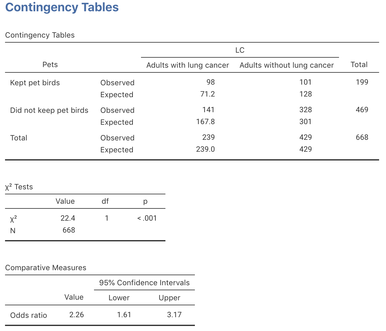
FIGURE 31.4: jamovi output for the pet-birds data
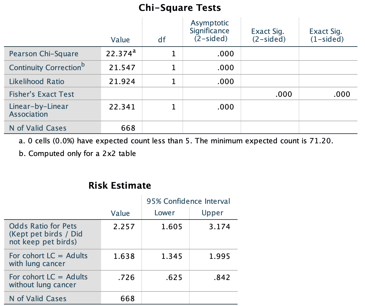
FIGURE 31.5: SPSS output for the pet-birds data