27.3 Sampling distribution: Expectation
A RQ is answered using data (this is partly what is meant by evidence-based research). Fortunately, for the body-temperature study, data are available from a comprehensive American study (Shoemaker 1996).
Summarising the data is important, because the data are the means by which the RQ is answered (data below).
A graphical summary (Fig. 27.1) shows that the internal body temperature of individuals varies from person to person: this is natural variation. A numerical summary (from software) shows that:
- The sample mean is \(\bar{x} = 36.8051^\circ\)C;
- The sample standard deviation is \(s = 0.40732^\circ\)C;
- The sample size is \(n=130\).
The sample mean is less than the assumed value of \(\mu=37^\circ\text{C}\)… The question is why: can the difference reasonably be explained by sampling variation, or not?
A 95% CI can also be computed (using software or manually): the 95% CI for \(\mu\) is from \(36.73^\circ\) to \(36.88^\circ\)C. This CI is narrow, implying that \(\mu\) has been estimated with precision, so detecting even small deviations of \(\mu\) from \(37^\circ\) should be possible.
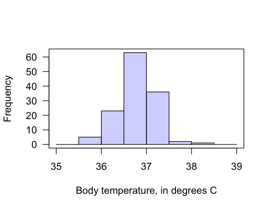
FIGURE 27.1: The histogram of the body temperature data
The decision-making process assumes that the population mean temperature is \(\mu=37.0^\circ\text{C}\), as stated in the null hypothesis. Because of sampling variation, the value of \(\bar{x}\) sometimes would be smaller than \(37.0^\circ\text{C}\) and sometimes greater than \(37.0^\circ\text{C}\).
How much variation in the value of \(\bar{x}\) could be expected, simply due to sampling variation, when \(\mu=37.0^\circ\text{C}\)? This variation is described by the sampling distribution.
The sampling distribution of \(\bar{x}\) was discussed in Sect. 22.2 (and Def. 22.1 specifically). From this, if \(\mu\) really was \(37.0^\circ\)C and if certain conditions are true, the possible values of the sample means can be described using:
- An approximate normal distribution;
- With mean \(37.0^\circ\text{C}\) (from \(H_0\));
- With standard deviation of \(\displaystyle \text{s.e.}(\bar{x}) = \frac{s}{\sqrt{n}} = \frac{0.40732}{\sqrt{130}} = 0.035724\). This is the standard error of the sample means.
A picture of this sampling distribution (Fig. 27.2) shows how the sample mean varies when \(n=130\), simply due to sampling variation, when \(\mu = 37^\circ\text{C}\). This enables questions to be asked about the likely values of \(\bar{x}\) that would be found in the sample, when the population mean is \(\mu = 37^\circ\text{C}\).
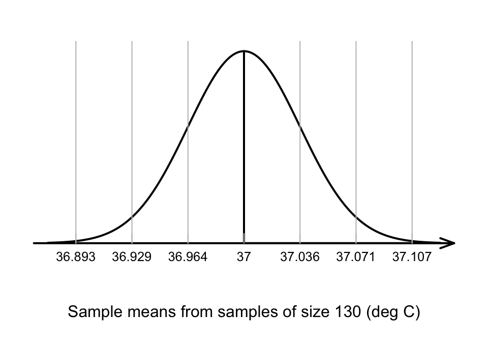
FIGURE 27.2: The distribution of sample mean body temperatures, if the population mean is \(37^\circ\)C and \(n=130\). The grey vertical lines are 1, 2 and 3 standard deviations from the mean.