17.5 Approximating areas using the 68–95–99.7 rule
Suppose again that heights of Australian adult males have a mean of \(\mu=175\)cm, and a standard deviation of \(\sigma=7\)cm, and (approximately) follow a normal distribution (Fig. 17.4).
Again, drawing the situation is helpful (Fig. 17.5).
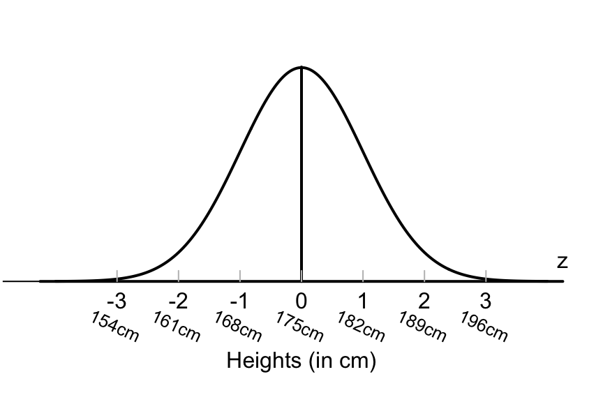
FIGURE 17.4: The empirical rule and heights of Australian adult males
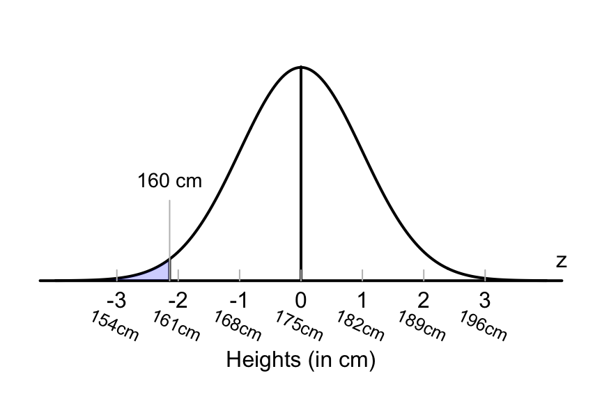
FIGURE 17.5: What proportion of Australian adult males are shorter than 160cm?
Proceeding as before, we need to ask ‘How many standard deviation below the mean is 160cm?’ Using Equation (17.1) to compute the \(z\)-score, \(160\)cm is
\[ z = \frac{160 - 175}{7} = -2.14, \] or \(2.14\) standard deviations, below the mean. What percentage of observations are less than this? This case is not covered by the 68–95–99.7 rule, though we can use the 68–95–99.7 rule to make some rough estimates.
About 2.5% of observations are less than 2 standard deviations below the mean (Example 17.1); that is, about 2.5% of men are shorter than 161cm.
So the percentages males even shorter than 161cm (that is, further into the tail of the distribution), will be less than 2.5%. While we don’t know the probability exactly, it will be smaller than 2.5%.
Estimates in this way are crude, but often serviceable. However, better estimates of ‘areas under the normal curve’ are found using tables compiled for this very purpose.
These tables are in Appendix B.2. ‘Percentages’ under a normal curve are also called ‘areas’ under the normal curve. The total area under a normal curve is one (or 100%), since it represent all possible values that could be observed.
We now learn how to use these tables, then come back to Example 17.5.