31.13 Exercises
Selected answers are available in Sect. D.29.
Exercise 31.1 Researchers (Christensen et al. 1972) studied the number of sandflies caught in light traps set at 3 and 35 feet above ground in eastern Panama. They asked:
The data are compiled into a table (Table 31.12), and summarised numerically (Table 31.13; partially edited) and graphically (Fig. 31.13). Use the jamovi output (Fig. 31.14) to evaluate the evidence, complete Table 31.13, and write a conclusion.In eastern Panama, are the odds of finding a male sandfly the same at 3 feet above ground as at 35 feet above ground?
| 3 feet above ground | 35 feet above ground | |
|---|---|---|
| Males | 173 | 125 |
| Females | 150 | 73 |
| Odds | Percentage | Sample size | |
|---|---|---|---|
| 3 feet: | ?? | ?? | 298 |
| 35 feet: | 1.71 | 67.3% | 223 |
| Odds ratio: | 0.67 |
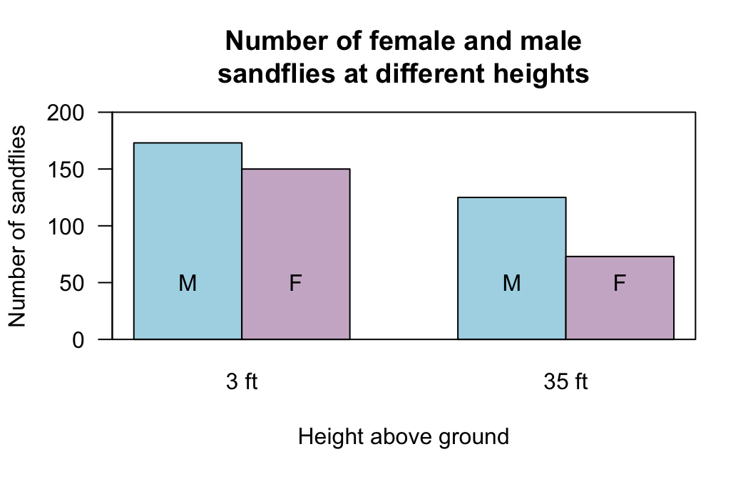
FIGURE 31.13: A side-by-side barchart of the sandflies data
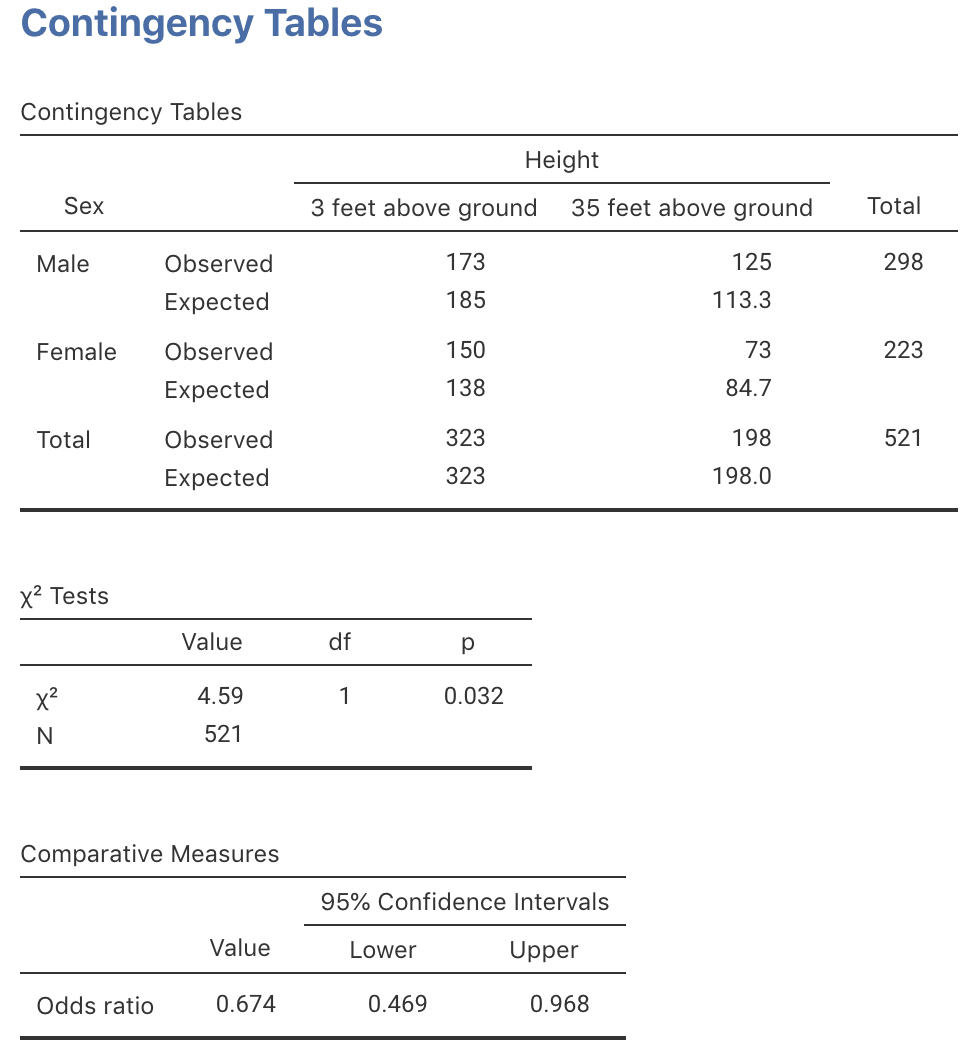
FIGURE 31.14: Using jamovi to compute a CI for the sandflies data
Exercise 31.2 A prospective observational study in Western Australia compared the heights of scars from burns received (Wallace et al. 2017). The data are shown in Table 31.14. SPSS was used to analyse the data (Fig. 31.15). (This study also appeared in Exercise 25.1, where the odds ratio, and the CI for the odds ratio, were computed.)
- Perform a hypothesis test to determine if the odds of having a smooth scar are the same for women and men.
- Write down the conclusion.
- Is the test statistically valid?
| Women | Men | |
|---|---|---|
| Scar height 0mm (smooth) | 99 | 216 |
| Scar height more than 0mm, less than 1mm | 62 | 115 |
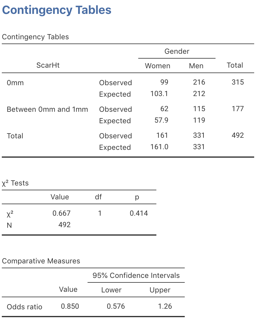
FIGURE 31.15: Using jamovi to compute a CI for the scar-height data
Exercise 31.3 In a study of turbine failures (Nelson 1982; Myers et al. 2002), 73 turbines were run for around 1800 hours, and seven developed fissures (small cracks). Forty-two different turbines were run for about 3000 hours, and nine developed fissures.
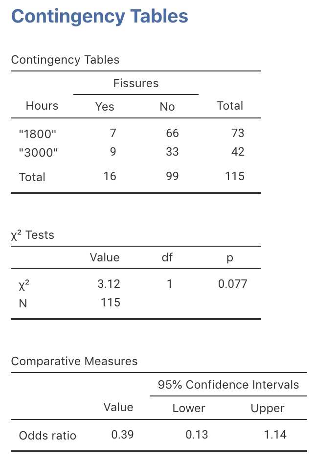
FIGURE 31.16: jamovi output for the turbine data
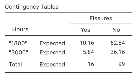
FIGURE 31.17: jamovi output for the turbine data: expected counts
Exercise 31.4 The Southern Oscillation Index (SOI) is a standardised measure of the air pressure difference between Tahiti and Darwin, and has been shown to be related to rainfall in some parts of the world (Stone et al. 1996), and especially Queensland (Stone and Auliciems 1992; Dunn 2001). As an example (Dunn and Smyth 2018), the rainfall at Emerald (Queensland) was recorded for Augusts between 1889 to 2002 inclusive, in Augusts when the monthly average SOI was positive, and when the SOI was non-positive (that is, zero or negative), as shown in Table 31.15. (This study also appeared in Exercise 25.4.)
- Using the jamovi output in Fig. 31.18, perform a hypothesis test to determine if the odds of having no rain is the same Augusts with non-positive and negative SOI.
- Write down the conclusion.
- Is the test statistically valid?
| Non-positive SOI | Positive SOI | |
|---|---|---|
| No rainfall recorded | 14 | 7 |
| Rainfall recorded | 40 | 53 |
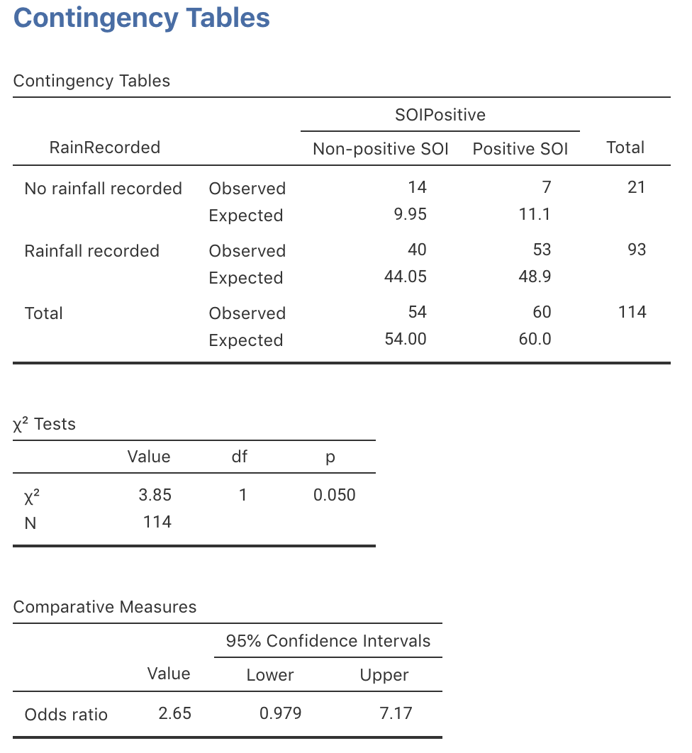
FIGURE 31.18: jamovi output for the Emerald-rain data
Exercise 31.5 A research study conducted in Brisbane (Dexter et al. 2019) recorded the number of people at the foot of the Goodwill Bridge, Southbank, who wore sunglasses and hats. The data were recorded between 11:30am to 12:30pm. Table 31.16 records the number of females and males wearing hats.
- Compute the percentages of females wearing a hat.
- Compute the percentages of males wearing a hat.
- Compute the odds of a female wearing a hat.
- Compute the odds of a male wearing a hat.
- Compute the odds ratio of wearing a hat, comparing females to males.
- Compute the odds ratio of wearing a hat, comparing males to females.
- Find the 95% CI for the appropriate OR.
- Using the SPSS output in Fig. 31.19, perform a hypothesis test to determine if the odds of wearing a hat is the same for females and males.
- Write down the conclusion.
- Is the test statistically valid?
| Not wearing hat | Wearing hat | |
|---|---|---|
| Male | 307 | 79 |
| Female | 344 | 22 |
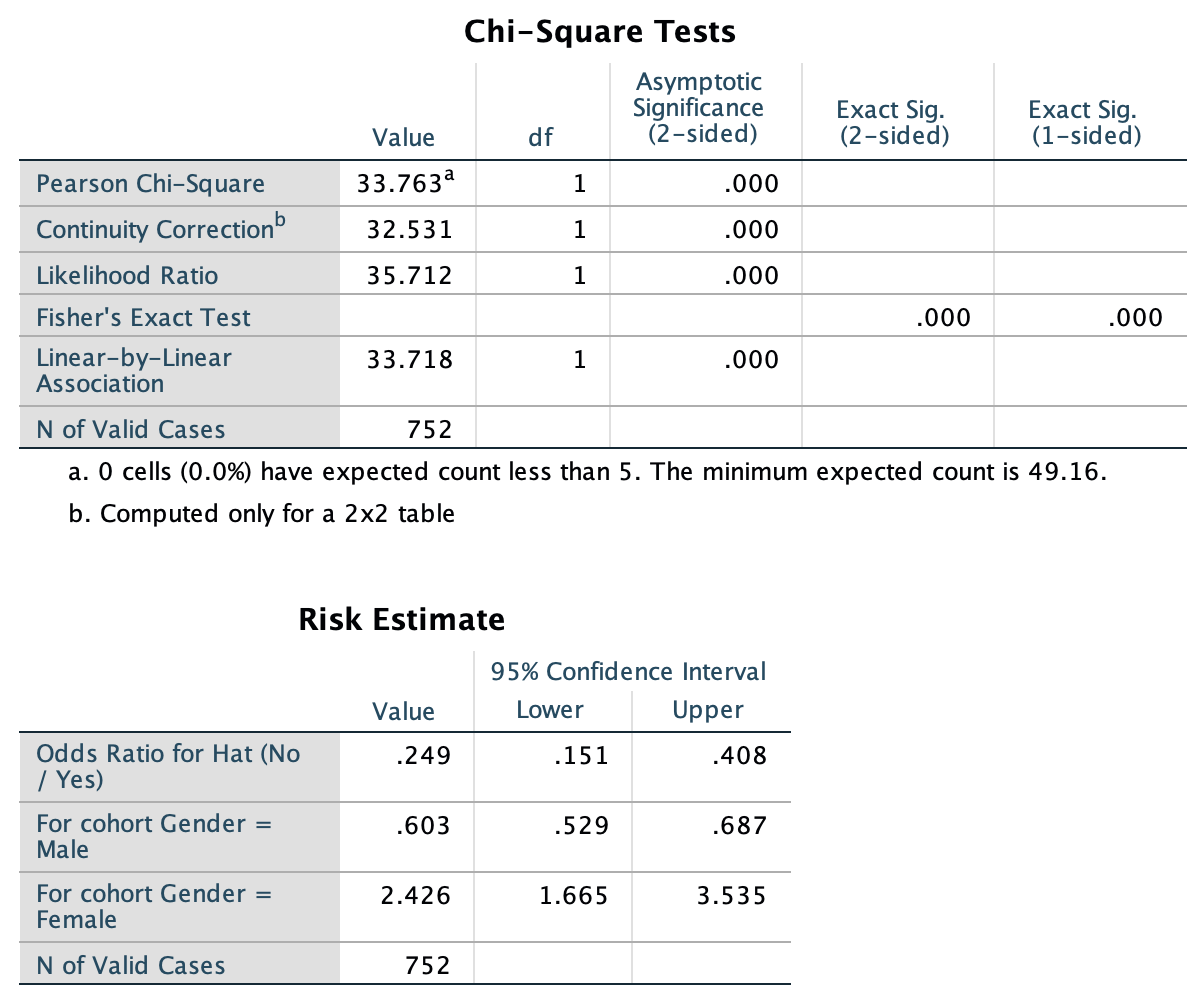
FIGURE 31.19: SPSS output for the hats data
Exercise 31.6 A study (Lennon et al. 2017) asked people about their mobile-phone interactions while crossing the road as pedestrians. Part of the data are summarised in Table 31.17.
- Compute the column percentages.
- Compute the odds of low exposure to each behaviour.
- Write the hypothesis for conducting a hypothesis test.
- Compute the expected counts.
- After analysis in jamovi, the value of \(\chi^2\) is 20.923 with two degrees of freedom. What is the approximately-equivalent \(z\)-score? Would you expect a large or small \(P\)-value?
- The \(P\)-value is given as \(P<0.000\). Write a conclusion.
| Answer call | Respond to text | Reply to email | |
|---|---|---|---|
| Low exposure | 263 | 259 | 302 |
| High exposure | 94 | 98 | 51 |