27.4 The test statistic and \(t\)-scores: Observation
The sampling distributions describes what to expect from the sample mean, assuming \(\mu = 37.0^\circ\text{C}\). The value of \(\bar{x}\) that is observed, however, is \(\bar{x}=36.8051^\circ\) How likely is it that such a value could occur by chance?
The value of the observed sample mean can be located the picture of the sampling distribution (Fig. 27.3). The value \(\bar{x}=36.8051^\circ\text{C}\) is unusually small. About how many standard deviations is \(\bar{x}\) away from \(\mu=37\)? A lot…
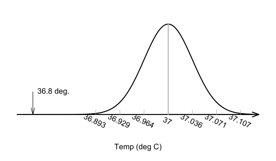
FIGURE 27.3: The sample mean of \(\bar{x}=36.8041^\circ\)C is very unlikely to have been observed if the poulation mean really was \(37^\circ\)C, and \(n=130\)
Relatively speaking, the distance that the observed sample mean (of \(\bar{x}=36.8051\)) is from the mean of the sampling distribution (Fig. 27.3). is found by computing how many standard deviations the value of \(\bar{x}\) is from the mean of the distribution; that is, computing something like a \(z\)-score. (Remember that the standard deviation in Fig. 27.3 is the the standard error: the amount of variation in the sample means.)
Since the mean and standard deviation (i.e., the standard error) of this normal distribution are known, the number of standard deviations that \(\bar{x} = 36.8051\) is from the mean is
\[ \frac{36.8051 - 37.0}{0.035724} = -5.453. \] This value is like a \(z\)-score. However, this is actually called a \(t\)-score because it has been computed when the population standard deviation is unknown, and the best estimate (the sample standard deviation) is used when \(\text{s.e.}(\bar{x})\) was computed.
Both \(t\) and \(z\) scores measure the number of standard deviations that an observation is from the mean: \(z\)-scores use \(\sigma\) and \(t\)-scores use \(s\). Here, the distribution of the sample statistic is relevant, so the appropriate standard deviation is the standard deviation of the sampling distribution: the standard error.
Like \(z\)-scores, \(t\)-scores measure the number of standard deviations that an observation is from the mean. \(z\)-scores are calculated using the population standard deviation, and \(t\)-scores are calculated using the sample standard deviation.
In hypothesis testing, \(t\)-scores are more commonly used than \(z\)-scores, because almost always the population standard deviation is unknown, and the sample standard deviation is used instead.
In this course, it is sufficient to think of \(z\)-scores and \(t\)-scores as approximately the same. Unless sample sizes are small, this is a reasonable approximation.So the calculation is:
\[ t = \frac{36.8051 - 37.0}{0.035724} = -5.453; \] the observed sample mean is more than five standard deviation below the population mean. This is highly unusual based on the 68–95–99.7 rule, as seen in Fig. 27.3.
In general, a \(t\)-score in hypothesis testing is
\[\begin{equation} t = \frac{\text{sample statistic} - \text{assumed population parameter}} {\text{standard error of the sample statistic}}. \tag{27.1} \end{equation}\]